Quasilinear oscillations in systems with large static deflections
Bạn đang xem bản rút gọn của tài liệu. Xem và tải ngay bản đầy đủ của tài liệu tại đây (9.62 MB, 30 trang )
P roceed ings of the International Confluence on A pplied Dynam ics H anoi, 20-25/11/1995
QƯASELINEAR OSCILLATIONS IN SYSTEMS WITH LARGE
STATIC DEFLECTIONS
N g u y e n V a n D a o
Vietnam National University, Hanoi
A bstract
In mechanical systems the static dcflcction of the clastic elements is usual not
appeared in the equations of motion. The reason is that either a linear model of
the clastic elements or their too small static dcflcction assumption was acccptcd.
In the. present paper both nonlinear model of clastic elements and their large static
dcficction arc considered, 30 that the nonlinear terms in the equation of motion
appear with different degrees of smallness. In this case the nonlincarxty of the sys
tem depends not only on the nonlinear characteristic of the clastic element but on
its static itflcction. The distinguishing feature of the system under consideration
is that if the clastic element had soft characteristic, the nonlinear system also be-
longs to the soft OTIC. If the clastic element has hard characteristic, the system
may be either soft or hard or neutral type, depending on the relationship between
the parameters of the clastic element and its static deflection.
The autonomous and non-autonomous system have been studied. Analytical meth
ods in combination with Computer have bttn used.
The problem of nonlinear oscillations of clastic structures with large static de
flection in general, and beams, plates in particular, may be studied in a similar
manner.
PART 1
1. Introduction
Let us consider the simplest oscillatory system which consists of a mass M
and the spring as shown in the F ig .l. The spring supporting the mass is
assumed to be nonlinear with the characteristic
/ ( u ) = C0U + /?0 U3 , (1 )
so that the spring force acting on the mass M is
c . ( A - * ) + / » . ( A - x ) 3 ,
where c0 is positive constant and /?„ is either positive (hard characteristic)
or negative (soft characteristic), A is the deformation of the spring at the
s t a t i c equilibrium position. ThÌ3 position is chosen aa the reference position.
W hen 1 = 0 , the spring force C0A + £0A3 is equal to the gravitational force
Mg, that is
-C0 A + /?0 A 3 = Mg.
M
umlreched
poiifion >
X
M
re ỉtren câ
ị
po sitio n
— — x.fl
F ig . 1
M easuring the displacement X from the static equilibrium position with
I chosen to be positive in the upward direction, and applying N ew ton’s
second law of motion to the mass M we obtain
M i + c0 2 + 3 £ 0 A 2x - 3/?0 Ax2 + /?„ I 3 = 0.
It is supposed that A is large and X is enough small, 30 that in comparison
with linear term, /90x3 is a small quantity of second degree and jS0A i 3 is of
the first degree of smallness:
= 0 (c), £ox3 = 0(e3), ậữ&x2 = 0 (ff),
2 _
where e is a small positive parameter. In this case Ax2 is finite.
Taking into account the viscous damping force h0x and exciting force P[t, z)
which are both assumed to be small quantities of second degree and intro
ducing the notation
2 c 0 + 3 & A 2 - ro
u =
— — , n = ~ r ,
M
M
= Ẽ2.
M '
(
2
)
we Can write the equation of motion of the mass M in the form:
X + <jj2 x = e~ỊX2 — e2(hx + f i x 3 — / ( t , i ) ) . (3)
In comparison with the classical Duffing equation, in the equation (3) the
small terms appear with different degrees, most of them are of second degree
of smallness. From the structure of the equation (3) one can predict that
the influence of the forces on the motion of the mass M can be found in the
second approximation of the solution. In the present paper a more general
equation will be investigated.
X + ui2 i = e-712 + c2F{r, < p (t),x , i),
(4)
19
ìere r is a slow tim e T = et, F(r, <p[r), X, x) is the periodic function relatively
ip w ith period 2rr which can be represented in the form
N
F[r,<plx,i) = ^2
n =-N
ie coefficients of this expansion Fn[r, X, i) are polynoms of X, X. It is
sum ed that the mom entary frequency i/(r) = is slowly changed over
at
e tim e and that Fn[T,x,x), u(r) have and enough number of derivatives
latively to r for all finite values of r. We will be specially interested in
e study of the resonance zone when w is near to - u, where p and q are
tegers.
A utonom ous system
rst, we study a special case of the equation (4) when F[r, <p(r),x, x) does
>t depend on time
F{t,ip[t)ix,x) = Q{x,x). (5)
)llowing to the a sy m p to tic method of nonlinear oscillation [l, 2] the solu-
an of the equation (4) in this case will be found in the form
X — a COS 0 + ffUi (a, 6) + e 2u2 (a, 6) + . . . (6)
here Ui(a, 0) are periodic functions of 6 with period 2ir which do not contain
e first harmonics sinớ, C08Ổ and
a, 9
satisfy the equations:
^ = cAi[a) + ff24 2(a) +
i t (7)
“37 = w + cBi (a) + ff2B 2(a) +
at
lbstituting these expressions into the equation (4) and comparing the
•efficients of e and c2 we have:
o2
w2 (-ggj- + Ui'j = 702 COS2 Ỡ + 2(UjjBi c os ỡ + 2uAi sin 6,
q 2
Ú1 (^~0Q2 U a) = 2 ^ 7 ^ ! C08 6 + Q (a C O S 0 , —aai sin i) +
+ 2au1B2 COS 0 + 2u) A-Ì sin 6 + R{ A\, Bi),
(8)
here R[0, = iZ(A1(0) = 0. Comparing the coefficients of the harmonica
I the first equation of (8 ) gives:
Ax = 0, Bi - 0, Ui = ^cos2ớ). (9)
Comparing the first harmonics sinớ and COS $ in the second equation of (8)
where (/) is averaged valued on time of the function /. We consider now
im portant examples:
E xam p le 1. D uffing equation
Supposing that Q(x, x) = -hi - fix3, we obtain
The oscillations are damped with the frequency depending on the am pli-
dd
tude. W ith the grow of time the momentary frequency -J- either increases
if a < 0 or decreases if a > 0 or is a constant if a = 0 . This is a, distin
guishing feature of the system with large static deflection. The parameter
a depends on the parameters c0, /?„ (spring) and A (static deflection).
The considered Duffing equation is modeled [3] on the computer for a con
crete case s = 0.25 in the system with hard characteristics p = 0.2 (Fig. 2).
On the phase plan there exist three degenerated points X\ = 0, x2 = 5.52
and 13 = 14.47, where z2 is a saddle point while X\ and I 3 are stable focal
ones. In the system with a soft characteristics p = - 0.2 (Fig. 3) the gener
ated points are Xi = -2.4 , X2 = 0, 13 = 3.4 where x-2 is a stable focal point
while the two other are saddle points.
E xam p le 2 . Van-der-Pol equation
It is assumed that Q(x, x) = —px3+ D { 1 —x2)i, where D is a positive constant.
We have
yields:
Ai = — — (sin dQ[a cos Ớ, — a u sin 0)),
(10)
( 11)
T hus, in the second approximation we have
where a and 6 are determined from the equations
da
dt
d6
dt
(13)
21
T
1
í
I
Ị
1
1
í
7
D uff ing e q u a t i o n (p =0.2)
2 0.0 000 X(t)
duffi ng equati o n <p=-0.2>
2 5 . 0 0 0 0
2 5 .0 0 0 0 X(t)
Fig. 3
id the equations of the second approximation are
The oscillation is self-excited w ith a constant amplitude a0 = 2. The es
sential difference in comparison with the classical Van-der-Pol oscillator 13
that the momentary frequency depends on the parameter Q which can be
either positive or negative or zero.
On the computer the Van-der-Pol equation has stable focal point I = 14.5
(Fig. 4) and a stable cycle with radius 2, which is independent from D > 0 .
I
■
*
I
u
/
/
V '
a n d erP o 1
/
( Q
■■■ ■!
1 1 V
e q u a tio n \ \
\ V -
_ \ A \
" v » . r s i w
1 I I 1
1
to
•
re
net
1I 0
I \ v *
\ V M
\ V -
f _ K W i .
• 2 0 . 0 0 0 0
1 ! \j \j \
Fig. ị
3. N o n -s ta tỉo n a r y n o n -a u to n o m o u a s y ste m
The approxim ate solution of the equation (4) in general case will be found
in the form
I = acos (-£ >+ + eui(r, a, VP, 0) + fi2u3 (r, a, ip,d) + , (15)
where s = -<p + rp and u, (r, a, <p, Ớ) are periodic functions of ¥?, 9 with pe-
7
riod 2jt and do not contain the first harmonics COSỔ, sinớ. The unknown
functions a and t/> satisfy the equations:
^ = e A i( r , a,4>) + c* A 2 [r, a, rp) + ,
d l _ _ (1 6 )
= u - -v[t) +cBi{rta,i>) + c2 B 3 (r, o, 4>) +
at q
By substituting the expressions (15) and (16) into the equation (4) and
23
mparing the coefficient of c and c2 we obtain:
2 / \ d 2 tiỵ d 2 U i n d 2 Ui 2
= ^a2 cos2 0 — — -y(r)) — 2awBi j COS
9
+ Ị(w - ~u{r))a~Q~p' + 2w-Ai] «in
o . « d^ll2 _ , . 3 2 U2 2 ^ 2 u 2 2
^ W a ^ + 2“ ‘'(r> f ^ + u' a*r+ " “a =
= 2 a 7 U i c o s ớ + F(r, <p, a COS Ớ, —aa; sin 0)
- [(“ - f "(r)) a7 ■ 2au,B2 + ^ 7 + Bl 3^r
. _ 3 5 i <9Bi 5 B i i
+ 2i4if?i + aA
1
—— + aBi — - + a —— sin 0
da ơr .
( 17)
- {2"frf* + 2l/(r)fra; + 2l/M A > Ũ ỹ
+ 2uAiÊdẽ + 2‘/[T)BlỆó ĩ + ĩuBl^p' (18)
+ L - p- v M )
V q v V dyị) dd dyị> da J d<p dr J
?he unknown functions j4i, Bi and Uj will be determined from the equation
17). By comparing the coefficients of harmonics in (17) we obtain:
Ai = 0 , Bi = 0, Ui = ( l - £ cos 2ớ) , 9 = -<p + v>. (19)
\jialogously, we can find A i , B i and u2 from the equation (18) for the
general form of the function F(rtip, x,x). However, we will concentrate
itten tion on two important cases:
Case 1 . T he p assage of the system throu gh the principal resonance zone
it is supposed that the function F(r, (p, X, x) is of the form
F(t,<p,x,x) = - h i - p x 3 + E sinip ự ), p = q = 1, (20)
where E is a constant. In this case the equation (18) becomes:
, , ><92 U2 „ . . 3 2 ti2 2 3 2 ti2 3
" ( r ) f ^ r + ỉ " ( ’ ) 3 ^ + " a i ? + w U ỉ =
= 2a~iui COS 9 + haw sin 9 — f3az COS3 9 + E sin <p(t)
3 A 2
— — v(r)) — 2aw.Ỡ2j C08 9
+ £(ui — v {T))a ~Q^ + 2cưAaj s in 9. (21)
dip
Comparing the coefficients of sinớ and C03Ớ in (21) we obtain
(w — v(r)) ~ I cluB i = - a a 3 — E ú n Ip,
d B
(u — v [t ) )cl— — + 2c jA 2 = — h a u — E COS t/>,
" d r p
a V ~ * Z '
Solving these equations we have
ha E /.
A 2 =
■ ■ C03 t/>,
2 CJ + i/( r )
_ a 2 £7
i?2 = — a + —
-
— — sint/;.
2cj a UI + y ( r )
(22)
Comparing the coefficients of the other harmonics in (21) and solving the
equation obtained we get
Uj = ĩ è ĩ ( ắ + f ) a3cos39- (23)
Thus, in the second approximation we have:
X = a COS Ớ + y r ( x ~ 3 cos 2d) ’ ^ = SP(Ế) -t- V-'(0 ) (2 4 )
where a and v> satisfy the equations:
4
d a 2
■/i £
— a +
r-r C08
d t 12 w + ^ (t) -I
drp e2a 2 e2£
- 7 - = UI - i/(r) + —— a"4 + —
— sin 1p.
dt 2u a u + v [t)}
(25)
These equations are solved on the personal computer by using the finite
C^h c E
difference method for the parameters —— = 0.5 • 103, —— = 0.158 • 10~3
U) UI
2 5
1 = + 0.1 (F ig .5), - - 0.1 (F ig.6) with the initial values: t = 0 ,
OJ w 3
= 10~ 6, v>0 = 0 . The parameter T) = — for Fig. 5 is rj = 0.97 + 10-6 i
r v e 1 , A t = 0 .0 4 ) , n = 0 .9 7 + 1 0 " 6t ( c u r v e 2 , A t = 0 . 4 ) , TỊ = 1 .0 3 - 1 0 _ 6 i
rve 3), r\ = 1.03 - 10“6i (curve 4) and for Fig. 6 is »7 = 1.02 - 10-6 t
rve 1), TJ = 1.02 - 10-5 i (curve 2), T) = 0.97 + 10-6 i (curve 3, A t = 0.04),
: 0.97 + 10-5 i (curve 4, At = 0.4).
e stationary am plitudes corresponding to the constant values of the fre-
ỉncy V are presented in the F ig .7 for the values mentioned above of / ,
and — + 0.1 (curve 1), a = 0 (curve 2), = - 0.1 (curve 3). The
ivy (dashed) lines in this figure correspond to the stability (instability)
oscillations.
mparing the Figs 5, 6 and Fig. 7 it is seen that increasing the velocity of
ssing through the resonance, the m axim um of the amplitude decrease and
s peak appear after the resonance peak. The maximum of the amplitudes
stationary oscillations is biggest.
Fig. 5
Fig. 6
I
Fig. 7
27
ise 2. P assing o f the Bygtem through th e param etric resonance
ỉsuming that the function F(r,ip, I, i) has the form
F[r, ip, X, i ) = —/ l i — fix3 + ex COB p = 1, q = 2 , (2 6 )
aere e is a constant. In this case the equation for determination of Ai, B2
id U2 is
2 . Ổ2 U2 , J 2 UJ 2 3 2 u 2 2
" M i ^ +2u,l/(r> a ^ +w + w “2 =
= 2a7Ui cos Ớ + haw sin 6 — 00? COS3 6 + ơa COS 6 COS <p
- Ị(w - ịu[r)) d- ệ ị - la u B iị COS 6
+ _|_ 2w A 3 | sin ổ. ( 27)
y comparing the coefficients of COS ớ and 8Ìn0 in (27) we have
/ 1 . .\ d Ả 2 „ o ca
-
2
~ 2au B 2 = - o a + Y cos 2V>,
/ 1 , N\ 5
$ 2
ca
CJ — - I ' M a —— + 2uii42 = —h a u
sin 2Ự>,
\ 2 / d\p q
3 572
here at = -0 — From these equations we obtain
4 6a/"*
(28)
^ ca • I
= — 2 ° — 2 ^ ( r ) 9
a a 2 c
B 2 =
-
7 - 7
cos 2t/>.
2a» 2 ỉ/(í)
ence, the equations of the second approximation become
da e2 / , ca \
i t = l \ ha+^T ),ia2V '
dip i / ( t ) e 2a 2 e 2 e
— = UJ
^— I- —— a 2 — -■ " COS 2V».
di 2 2ai 2ỉ/(r)
'hese equations are solved on the personal computer for the parameters
- ị = 8.9- 1CT3, — = 0.002 and ^ = 0.02 (Fig. 8), ^ = - 0.02 (Fig. 9)
(jJ* (J (jJ* _ ^
nd w ith the initial condition t = 0 , a0 = 0.09, v>0 = 0- F °r the case of Fig. 8 :
= = 1 + 10-6 t (curve 1), ụ. = 1 + 2 • 10-5 f (curve 2) and for the case of
ig.9: fi — 1 — 10-6 i (curve 1), /I = 1 — 2 • 10-6 i (curve 2).
(29)
Fig. 8
Fig. 9
29
\.RT n
L this part two following problems have been examined:
I The non-linear oscillations of electrom echanical systems with limited
Dwer supply and large static deflection of the elastic elements.
I The interaction between the self-excited and parametric oscillations and
so between the self-excited and forced ones in the non-linear systems with
.rge static deflection of the elastic elements when the mechanisms exciting
lese oscillations coexist.
1 both problems there is a common feature characterized by the fact that
le nonlinearity of the system under consideration depends on the parame-
:rs of elastic elem ents and their static deflection and by the appearance of
ie non-linear terms with different degrees of smallness in the equations of
lotion. Stationary oscillations and their stability have been paid special
ttention.
NONLINEAR OSCILLATIONS OF THE SYSTEM WITH LARGE STATIC DEFLECTION
F THE e l a s t ic e l e m e n t s a n d l im it e d p o w e r s u p pl y
1 this section the non-linear oscillations of a machine with rotating unbal-
nce and large static deflection of the non-linear spring and limited power
apply are considered. The equations of motion of the system under consid-
ration are different with those of classical problem [5] by the appearance of
le non-linear terms with different degrees of smallness. This feature leads
D the dependence of the hardness of the system no only on the parameters
f the elastic element but also on its static deflection.
'he results obtained are different in both quality and quantity with those
btained by Kononenko V. o . [5]
. Equations of m otion
ig. 10 illustrates a machine w ith a pair of counterrotating rotors of equal
nbalance (so that horizontal components of the centrifugal force vectors
ancel), isolated from the floor by non-linear springs and dashpots with
a m p in g c o e fficien t h0
’he springs supporting the mass assumed to be negligible in mass w ith a
on-linear characteristic function:
-'here c0 is a positive constant, Po is either positive (hard characteristic) or
egative (soft characteristic). The deformation of the spring in the static
quilibrium position is A, and the spring force C0 A + /90A 3 is equal to the
ravitational force m0g acting on the mass:
(30)
(31)
Fig. 10
where m0 = ml + m is defined as the sum of the main mass m l and the ro
tating unbalance m asses m, that is the total mass supported by the springs.
The displacement X is measured from the static equilibrium position with
I chosen to be positive in the upward direction. All quantities - force,
velocity, and acceleration - are also positive in the upward direction.
The system under consideration has two degrees of freedom and the gener
alized coordinates I and <p completely define its position.
The kinetic energy of the system under consideration is
T 2 + 2 ”
Zrr
= X + r COS
ip , 2 m
= r sin
<p.
Hence
T = - m i 2 — m r x < p sin ip + - I< p ^ , I = m r 2 . (32)
2 u 2
For the potential energy, the reference can be chosen at the level of the
static equilibrium position:
u — — (A — x)2 + —(A — x)* + m0 gx + mgr COS <p. (33)
2 4
The Lagrange’s equations give
I<p = mrx sin. (p + mgr sin <p, (34)
m 0x + cax + ^ 0x3 4- 3/30 A 2i — 3£ 0 A x 2 = mripsin ys + mr<p2 C03 !£>.
Taking into account the driving moment £,(<£) and the frictions H[<p), k0x
we have the following equations of motion:
lip = L[<p) — H[<p) + mrx sin + m jr sin <p,
m 0r + c0x + /i0x + £ 0x3 + 3£0A 2x - 3 £ 0Ax2 =
= mr£ sin + mrv?3 COS £>. (35)
31
ipposing that A is rather large and X is enough small, SO that P0X3 is a
lall quantity of second degree (e2), while is of first degree (e), where
IS a small positive parameter. Obviously, in this case £0A2X is finite.
is assum ed also that — < 1. ^ < 1. The friction forces, the forces
m 0 I
r<p7 CO8<p, mrtp sin <p and the mom ents mrxsinip, mgr sin ip are supposed to
i small quantities of é1.
hus, we have the following equations of motion:
The equations (36) are different with those in Kononenko V. o . work [5] by
he appearance of the quadratic term C7 X2 and by the degrees of smallness
if the terms. These equations characterise the systems with weak excitation
ind large static deflection.
Ì. Solution
iVe limit ourselves by considering the m otion in the resonance region, where
;he frequency u of the free oscillation is near to the frequency n = <p of the
,'orced oscillations.
We shall find the solution of equations (36) in the series [l]
where Ui[a,rp,ip) do not contain the first harmonics cosrp, sinrp, = <p + 0
and are periodic functions of rp and <p with period 2ir, and a, 6 are functions
satisfying the equations
ỷ = e2 [Ml (v?) + q(x + g) sin <p],
X + W2Z = e'jx3 + e 2 (pip sin <p + p<p2 COS <p — h i — fix5),
(36)
here
(37)
I = a cos(y? + 6) + eu x ( a , ĩp, <p) + e 2 u 2 (a , <p) + ff3
(38)
(39)
The first equation of (36) is then
= e2 [Mi. (n) + q(x + g) sin <p].
(40)
32
To determine the unknown functions Ai, Bi, U,- we differentiate the expres
sion (38) and substitute it into (36). We have:
X = — OU) 8in
( du\ <9ui i
in rp + eI — ai?i sin V’ + Ai COS t/) + CJ + n 1
of — 3ui du 1
+ t { — aB<2 sin yị) + Ả2 COS yịỉ + B\ -“ T + Ax -T-
l dw da
dyị)
n 5 u ?_\ , 3
+ “ s f + n a f l + e
X = — CLOJ COS 0 + tf I Ị(u/ — n) — 2awBij COS t/i — Ị(u — n)
1 • / _o 5^U1 <92 U1 2 (92ux i
+ 2w A ij sin t/i + n ! ^ - + 2 u ; n ^ + u ,
+ e2| [(w - n)-QQ- - 2auiB2 costp - (c j-H )a ^ -
+ 20JA2J sin ý + (^A\ ~qq' — a -^i) cos 0 - {^A \B
dB 1 5 B i\ d2u, <32u,
+ ^ + aBl sin ^ +2 n + 2uM 1
dB i
dd
_ <92tii 32ut dB\ <9tt 1
+ i n f l l 3 ^ + 2" B l 3 ^ + l" ~ n ) « s v r
, 3 u i / 2 ^ 3 U2 _ 5 2 U2 2
+ (“ - n)IT !7 + n 3 ^ +2a,na ^ +,J
+ *3 . . .
d 2 U2
d\p2
}
(41)
Substituting the expression (41) into the equation (36) and comparing the
coefficients of e and ff2 we obtain:
/_ 3 d
\ 3
2
r. <9i4i _ ,
( n — h w ) U[ +u Ui + (w — n) —
-
2auiBi COS 0
\ ơ<p Ơ 0 / L ƠƠ
r <95
— 1^(0; — n)a dg + 2u/y4i] sin v> = 7 a2 COS3 ự),
(42)
/- d 3 \ J 2 r, dA- 2 _ 1
(na^+“ aV) U3+w “J + r ' - n> gf~ 2 .
r dB 1
— I^u — n)a d
02
+
2
oj^
4
.
2
j sin rp = —R(A\, B\)
cos \Ị)
■+■ 2~jaui COS t/> — ^a
3
C033 i/> + ^OOJ sin v> ■+■ pH
2
COS Ip,
where J?(0 , Si) = R{AU 0) = 0.
(43)
33
)mparing the coefficients of the harmonics in (42) we have
(w - ĩì)~ỹỹ' - 'la uB ị = 0 ,
(w - + 2wAi = °»
/_ d d \ 2 2 2 2
Ịn— + U1 + w «x = 7° cos 0
itions yields
2 , 1
)lving these equations yields
Ai=0, Si=0, Ui = ^ 2 ( l - £ cos 2V>). (44)
omparing the coefficients of the first harmonics sin t/>, COS 4> in the equation
3) we have
_ n ) - 2auBi = ^ ^
+ p H 2 COS 6,
uu D u* 4
d Đ
(cư — n ) a — - 4- 2u»i42 = —/law — pfl2 sin 0.
dd
:om these equations one obtains:
ha pfl2
j42 =
— sin 6 .
2 2 (j + n
n _ 1 / 3 a 5 'T2 \ 2 p ° 2
ỉ t ĩ ) a ~ ĩ^ + n ũ cos
(45)
he equation for determination u2 is
(nỂ + “ Ẩ;) 3“2 + “2“2 = - ( ả + f ) °3 cos ^
ence
U2=iih(f+ Ể ) a5c053,>' {46)
hus, in the resonance zone n « w we have the following equations in the
icond approximation
X = GC08(¥J + i ) + f f ( ^ 2 - ^ ã 0 0 8 2 ^ ) ’ (4 7 )
here n, a and 0 satisfy the equations
Ệ = ^ [ M i ( n ) + i ^ » o . i n « ] ,
d ; = " 2 ẳ i (“ '“ I + ', n 2 “i" '') ' (4 8 )
de _ 1 r. o 'V n 2 \
^ = n h - n _ ^ r cosS)'
■vhere
L_ 2 _ 1 / 3 _ 5 * 7 f 4 QA
The stationary solution of the equation (48) is determined from the rela-
dỉì da dớ
tions — = 0 or
dip dip d<p
M i( n ) + - g w 2 a s in ổ = 0,
haw + pf)2 sin# = 0, (50)
w e - n — e 2 — COS 9 = 0.
2 ua
Eliminating the phase 9 from the la3t equations of (50) we obtain
t t V ,n ) = 0 , ' (51)
where
I^(a2, n) = w2a2[ff4À2 + 4(we - n)2] - c 4p2n4. (52)
In the resonance zone n RJU, the equation (51) gives approximately
.2 _._2 . .2 . I p2uji L2. .2
w + cẦa a Ẩ ± i i \ J r- T - - h i ujẦ . (53)
From this relation it follows that the non-linear oscillation has:
- a hard characteristic (Fig. 7x) if Q > 0 or if
c0 >ĩ/3ữz 2 (54)
- a soft characteristic (F ig.72) if
c0 < 7/90A2, (55)
- a linear characteristic (Fig. 73) if
ca =7ổ 0A2. (56)
Eliminating 6 from the first two equations of (50) we have
L(n)-S(n) = 0, (57)
where
5 ( n ) = t f ( n ) - f ^ 0a2. (58)
The equation (51) is sim ilar to that in the system with ideal power supply
[4]. The difference is that n should be satisfied the relation (57) which can
be solved graphically as shown in fig. 11
35
Fig. 11
3. Stability of stationary oscillations
Equations (50) can give some stationary values n = n 0, a = a0, 6 = 60. To
study the stability of these values we introduce a perturbation of n, a and
Ĩ:
sn = n - n 0) Sa — a — a0, 6d = 6 -d 0.
We denote the right-hand sides of the equations (48) by 4>n(n, a, Ổ),
i>12(n, a, S), $ i 3(f], a, 9) respectively. Below, the derivatives will be calculat
ed at the stationary values of n, a and 6 which satisfy the relations (50).
We have the following variational equations:
dsti
J " = bnỏíì ■+■ biiSa, + bizSO t
dip
—— = ỏ2i ^ í ì + 6226a + bisSO t ( 59)
dip
dse
—— = bsiSÍÌ •+■ 6326a -ị- b33S0,
dip
where
6
1 _ c?$13
t>23 = Q í 01'* - n ) a ' 6 3 1 =
= i ( n - 2 w e),
an n2V '
b 32 —
13
5 a
_1_
r d / > o
y-(awe) - n
Ida
i>33 —
13
30
2mon
The characteristic equation of the system (59) is
A3 + Dị + £?2-^ -1“ -^3 =
where
D i = — (6U + ồ23 + 633),
D 2 = 611633 + &11&22 + ỉ>22^33 - ^32^23 - &12^21 — ^13^311
Dz — &11&23&32 + ^12^21^33 + ^13^22^31 ~ ^11^22^33
— 612^23^31 - 613621632-
The R uth-H urw itz’s criterium of stability is
D\ > 0 , z?3 > 0, D\D2 ~ Dz > 0 .
We have
m 0 n /Q
As usually, it is supposed that -^rL(Q) is negative and ~xH{Vi) is positive,
a u a li
30 that /V is negative. Hence, Di is always positive.
The second stability condition Ữ3 > 0 as shown by Kononenko ’5’ is the
most important one. This condition is equivalent to the inequality
(61
(62)
(622ỏ33 - Ò23632) a’ < ^
(63
where = $ u (n, a(n), Ớ(Q)) and o(n), Ớ(D) are found from the last two
equations of (50); namely
* Ĩ 1 = j ^ [ £ ( n )-s(f i) ].
It is easy to verify that
^22^33 ~ ^23^32 — 0-2
dw
da2 ’
where w is of the form (52) and Ơ2 is a positive constant. Now, the stability
condition (63) can be represented in the form
(64)
37
dW
is noted that — - > 0 is the stability condition of stationary oscillation
dor
dW
hen ft is a given constant. is positive on the heavy branches of the
o a
ĩsonant curve. The sign of the derivative
G = ^ [ L ( n ) - s ( n ) ] (65)
an be obtained by considering the relative positions of the graphs L(n)
nd 5(0).
or the case of the system with a hard characteristic (Fig. 11) it is clear
bat G is negative at points Rx, R2 and ÌỈ3, 80 that the points i?i and i?3,
d \v
/here —— is positive, correspond to the stability of stationary oscillations.
da
^he point R2 corresponds to the instability of stationary oscillations, where
)W .
— IS n eg a tiv e.
ia*
n comparison with a system with an ideal energy source [4], the unstable
iranch of the resonance curve remains the same. But the jump phenomenon
ccurs in a different manner. As n is increased the amplitude of oscillation
/ill follow the solid arrows and the jump in the amplitude will take place
rom p to Q. W ith a decrease in frequency fi the amplitude will follow the
[ashed arrows and the jump will be from T to u. The points of collapse p
.nd T are the points of contact of the characteristic L(n) and the functions
’(H).
'or the case of the system having a soft characteristic (Fig. 12), the part
>f the resonance curve indicated by the dashed (heavy) line corresponds to
he instability (stability) of stationary oscillations, provided the frequency
dW I dW \
1 is a given constant. On this part —— < 0 . ( — - > 0 . The sign of the
dáị '
lerivative G (65) depends on the slope of the characteristic, i.e. on the
juantity -j^-L(Cl). It is necessary to distinguish two cases:
dll
i) when the characteristic is steep, i.e. -~L{Ĩ)) has a large absolute value
dll
Fig. 12)
Ỉ) when the characteristic is gently slopping, i.e. — L{ft) has a small ab
solute value (Fig. 13).
[n the first case the derivative G (65) will be negative on the parts PU,
PT and TQ (Fig. 12). Therefore, the stability condition (64) will not be
dW
satisfied on PT , where < 0 , but it will be satisfied on PU and QT;
d a 0
dW
where —— > 0 .
In the second case, the derivative G (65) will be positive on the parts PƯ
ind PT and negative on QT. Therefore the condition (64) is satisfied on
3T P and is not satisfied on PU (Fig. 13).
Fig. 12
II. w e a k i n t e r a c t i o n b e t w e e n t h e s e l f - e x c i t e d a n d p a r a m e t r i c os c il
l a t i o n s IN THE SYSTEM WITH LARGE STATIC DEFLECTION
The present section deals with some related problems when two mecha
nisms exciting the self-sustained oscillation and parametric one coexist in
one system. Following the assumptions in [41, these oscillations are weak
They appear only in the second approximation of the solution and their
interaction is weak, also.
In comparison with the classical problem on the interaction between self
excited and parametric oscillations [6], the system under consideration has
distinguishing feature which is characterized by the fact that its non-linear
ity (hardness, softness) depends on the parameters of elastic element and
its static deflection. Namely, when the initial system has a hard character
istic, the resonance curve may belong to a soft type. Therefore, the results
obtained are different with the classical ones both in quality and quantity.
39
Equation of m otion and approximate solution
ing the assum ptions and notations in the previous paper [4] we study
: oscillations described by the equation:
X + ú 2X = e-yx2 — e2[^ z3 + D (ơX1 — l ) i — ex COS i/t\, (66)
ere w, 7 , h, /?, D, e, Ơ and V are constan ts, D > 0, <7^ > 0, u > 0, V > 0,
• 0, Ơ > 0, c is a sm all positive parameter.
IS su p p os ed th a t V is in the neighb ourho od o f 2(Jj (p aram etric resona nce),
hen D = 0 equation (66) describes the system with parametric excitation,
hen c = 0, equation (66) represents a self-excited oscillator.
ie parametric and self-excited oscillations have a common feature that
i origin X = X = 0 is unstable. Under the resonance condition these
:illators may have a certain interaction.
ie solution of the equation (66) is found in the form
I = a COS 6 + cuxỊa, <p, 6) + c2u2(a, <p, Ớ) + e3 , (67)
lere 9 — — + Tp, <p = 1 /t and u, are periodic functions of <p and 8 with period
w h ich do no t co n tain the first harm onics COS 6 and sinớ. T he u n k n o w n
ictions a and ĩp are determined from the equations
^ = c A ^a , v») 4- e2A2[a, rp) + ,
di (68)
^ 7 = w ” 2 + + (a , v») +
bstituting the expressions (67) and (68) into equation (66) and comparing
i coefficients t and £2 we obtain:
[ v -
«1 + W2U1 = Tfo2 co s2 Ổ (6 9 )
\ d<p 96 /
9Ai _ 1 r / u\ dB\
" 2 ) a * ~ 2 a u B ll c o s e * l r " 2 ) a a ệ + 2 u A l
h w — Ị u 2 + w 3 u 3 = 2(171*! COBÍ + F[<pt a c i
- [(“ ~ 2 ) ^ C0s9+ [(“ ■ ì ) aÊỆ
+ iỉ( Ax, Bi)
sin 0,
( 1/ —— + w u 2 + w 2u 2 = 2a~fUi COS 0 + F[<p) a COS Ớ, —aui sin 0)
dB2
+ 2 cưẨ 2
(70)
lere
<p = vt, R [0 , f? i) = i ỉ( i 4 i ,0 ) = 0,
F{tp, X, i ) = — [/?x3 + D (ơx2 — l ) i — c x c o s v=»], (71)
a cos 6, —CLU1 sin 6) = F[tp, I, i)
CO* 9
i s - t w I in 9
( “ " 2 ) B~ a t - 2°“ B l =
( " - ỉ ) a^ ' + 2" '4l = 0' (72)
I d 3 \ 2 2 22/1
V d + u dd) Ul + ui = 7a cos 9-
These equations give
Ax = Bi = 0, «i a s 2 £ _ ( i - ỉ c o . 2 í ) l ớ = ^ í + 0. (73)
C o m parin g the coefficients of the first harm onics sin 0 and COS 9 in (70) yields
Comparing the coefficients of the harmonics in (69) we have
f u\ d A-2 3 s ,
( w
“ T -;
2 a w 5 j = - a a + - a COS 20 ,
\ 2 / arp 2
Ị w \ d -Ỡ2 ( era2 \ e
m — — a —
h 2w ^42 = awl? 1
— - a sin 20
\ 2/ drp \ 4/2
ft = i/9 -Ẽ 2l
4 6w2
So lving these equations we obtain
aD ( a a? \ ea .
2 I 1 - 4 ) ~ 21/
_ a -> «a
a i ?2 = — a — —-COS 2^1.
2w 2i/
T h u s, we have in the second approxim ation
X = OCOS0 + ( l - ^C03 2 ớ ), ÍJ = 2 Í + ^’
(74)
/ 0
2w3 V 3 '
■ /■ era2 \ ea .
a£) ( 1
— I — — sin 21/1
\ 4 / 1 /
-2 ,_._3
a
cia ff2
= y
d\Ịj ( v\ t‘ I aa~ ea \
—— = w — — ) a + — ——
— cos 2 0 ) .
dt \
2
)
2
\ u V J
(76)
2. Stationary’ oscillations and their stability
Equation^-(76) have a triv ia l solution a = 0. The non trivia l stationary
am plitu de a0 and phase \Ịi are determined by equations ^ = 0, — = 0 or
at dt
( ƠCL2 \
2ụjjjDyl
— J = csin2 </>0,
4 ụ u (^1 - + — a'J = í c c o s 2 t/>0 ,
41
sre /i 5= — . E lim in a tin g the phase Tp0 gives
2uj
WCo„pi.) = 0, (77)
0 0 ’ + ^ (l - - ĩỆ ^ I • <78>
)m relation (77) we find approxim ately:
= i + ^ 4 v S - ^ - 4 ) - (79>
is form ula is plotted in the figure 14 for the param eters
2 u 2
= 1.5 • 10—3, — = 10~3, Ơ = 40,
u
c‘ a
u;2
= 0.01 (curve l) and a = 0 (curve 2)
ability of the statio nary solution obtained is investigated by using the
n a tion a l equations. Denoting the right hand sides of the equations (76)
p and Q , respectively, we have
( £ ) . - * ? ■ O r ^ - 4 ) ’
lere the su b script “o” means that the derivatives are calculated for sta-
inary values a0, rp0. T h e stability conditions are
snce, we have
« : > * . ( « »
the figure 14 the heavy (dashed) branch corresponds to the sta bility
n stab ility) of stationary solution where the inequalities (80) are satisfied.