Flatness, Backstepping and Sliding Mode Controllers for Nonlinear Systems
Bạn đang xem bản rút gọn của tài liệu. Xem và tải ngay bản đầy đủ của tài liệu tại đây (571.85 KB, 22 trang )
Flatness, Backstepping and Sliding Mode
Controllers for Nonlinear Systems
Ali J. Koshkouei
1
, Keith Burnham
1
, and Alan Zinober
2
1
Control Theory and Applications Centre, Coventry University,
Coventry CV1 5FB, UK
{a.koshkouei, k.burnham}@coventry.ac.uk
2
Department of Applied Mathematics, The University of Sheffield, Sheffield S10
2TN, UK
1 Introduction
Sliding mode control (SMC) is a powerful and robust control method. SMC
methods have been widely studied in the last three decades from theoretical
concepts to industrial applications [1]-[3]. Higher-order sliding mode controllers
have recently been addressed to improve the system responses [1]. However, when
designing a control for a plant it is sometimes more beneficial to use combined
techniques, using SMC in conjunction with other methods such as backstepping,
passivity, flatness and even other traditional control design methods including
H
∞
, proportional-integral-derivative (PID) and self-tuning. Note that PID con-
trol design techniques may also be used for designing the sliding surface. A
drawback of the SMC methods may be unwanted chattering resulting from dis-
continuous control. There are many methods which can be employed to reduce
chattering, for example, using a continuous approximation of the discontinuous
control, and a combination of continuous and discontinuous sliding mode con-
trollers. Chattering may also be reduced using the higher-order SMC [4] and
dynamic sliding mode control [4, 5].
When plants include uncertainty with a lack of information about the bounds
of unknown parameters, adaptive control is more convenient; whilst, if sufficient
information about the uncertainty, such as upper bound is available, a robust
control is normally designed. The stabilisation problem has been studied for dif-
ferent classes of systems with uncertainties in recent years [6]-[10]. Most control
design approaches are based upon Lyapunov and linearisation methods. In the
Lyapunov approach, it is very difficult to find a Lyapunov function for designing
a control and stabilising the system. The linearisation approach yields local sta-
bility. The backstepping approach presents a systematic method for designing a
control to track a reference signal by selecting an appropriate Lyapunov function
and changing the coordinates [11, 12]. The robust output tracking of nonlinear
systems has been studied by many authors [13]-[15]. Backstepping technique
guarantees global asymptotic stability. Adaptive backstepping algorithms have
G. Bartolini et al. (Eds.): Modern Sliding Mode Control Theory, LNCIS 375, pp. 269–290, 2008.
springerlink.com
c
Springer-Verlag Berlin Heidelberg 2008
270 A.J. Koshkouei, K. Burnham, and A. Zinober
been applied to systems which can be transformed into a triangular form, in
particular, the parametric pure feedback (PPF) form and the parametric strict
feedback (PSF) form [12]. This method has been studied widely in recent years
[11, 12], [15]-[19].
If a plant has matched uncertainty, a state feedback control may stabilise the
system [7]. Many techniques have been proposed for the case of plants contain-
ing unmatched uncertainty [20]. The plant may contain unmodelled terms and
unmeasurable external disturbances bounded by known functions or their norm
is bound to a constant.
SMC is a robust control method and backstepping can be considered to be
a method of adaptive control. The combination of these methods, the so-called
adaptive backstepping SMC, yields benefits from both approaches. This method
can be used even if the system does not comprise of an unknown parameter. The
backstepping sliding mode approach has been extended to some classes of non-
linear systems which need not be in the PPF or PSF forms [15]-[19]. A symbolic
algebra toolbox allows straightforward design of dynamical backstepping control
[16]. A backstepping method for designing an SMC for a class of nonlinear system
without uncertainties, has been presented by Rios-Bol´ıvar and Zinober [16, 17].
The adaptive sliding backstepping control of semi-strict feedback systems (SSF)
[21] has been studied by Koshkouei and Zinober [22].
In this chapter, a systematic design procedure is proposed to combine adaptive
control and SMC techniques for a class of nonlinear systems. In fact, the back-
stepping approach for SSF systems with unmatched uncertainty is developed. A
controller based on SMC techniques is designed so that the state trajectories ap-
proach a specified hyperplane. These systematic methods do not need any extra
condition on the parameters and also any sufficient conditions for the existence
of the sliding mode to guarantee the stability of the system.
On the other hand, flatness is an important property in control theory which
assures that the system can be stabilised by imposing an artificial output [23]-
[25]. A linear system is flat if and only if it is controllable. A SISO system with
an output is not flat if the relative degree of the system with respect to the
output (if it is defined and finite) is not the same as the order of the system.
In general, there is no comprehensive systematic method for classifying flat and
non-flat systems, and also for finding a suitable flat output for nonlinear systems.
However, the controllability matrix yields a flat output for a linear system [23]
and flat time-varying linear systems have been studied by Sira-Ram´ırez and
Silva-Navarro [26]. In addition, the control of non-flat systems is an important
issue which has been studied since the last decade [24, 27, 28].
Flat outputs may not be the actual outputs of the system. Flatness for the
tracking problem of linear systems in differential operator representation has
been considered by Deutscher [29]. For MIMO nonlinear systems, there are dif-
ferences between exact feedback linearisablility and differential flatness (for ex-
ample see [24, 28]). However, most published papers have dealt with flatness or
non-flatness of SISO systems.
Flatness, Backstepping and Sliding Mode Controllers for Nonlinear Systems 271
Exact feedforward linearisation based upon differential flatness has been stud-
ied by Hagenmeyer and Delaleau [30] in which a flat system is linearised via
feedforward control using the differential flatness trajectory satisfying a certain
condition on the initial conditions. In fact there is a relationship between the flat-
ness and linearisability of nonlinear systems by feedback. In particular, for single
input systems, flatness is equivalent to linearisability by static state feedback
and static feedback linearisability is equivalent to dynamic feedback linearisabil-
ity [31]. In other words, linearisation via static (dynamic) state feedback and
coordinate transformation is equivalent to the linearisation by the static (dy-
namics) feedback of some outputs and a finite number of their derivatives. The
practical and asymptotic tracking problems for nonlinear systems when only the
output of the plant and the reference signal are available has been considered in
[32]. In addition the concept of global flatness has been presented. A system is
not globally flat if either the relative degree of the associated augmented system
is not well-defined everywhere or the change of coordinates using a particular
transformation is not a global diffeomorphism [32].
SMC and second-order SMC for nonlinear flat systems are also considered
in this chapter. The method benefits from the advantages of both approaches.
The important and main property of SMC is its robustness in the presence of
matched uncertainties whilst the flatness property guarantees that the control
can be obtained as a function of the flat output and its derivatives. In this
case, the sliding surface is also introduced in terms of the flat output and its
derivatives.
Differential flatness property and the second-order SMC for a hovercraft vessel
model has been studied in [33]. The technique has been proposed for the spec-
ification of a robust dynamic feedback multivariable controller accomplishing
prescribed trajectory tracking tasks for the earth coordinate position variables.
Moreover, in this chapter a gravity-flow tank/pipeline system is stabilised via
an SMC obtained from flatness and sliding mode control theory. This combined
method inherits the robustness property from SMC. If sufficient information
about the flat output is available then the control is accessible and applicable
without requiring further knowledge of the system variables.
This chapter is organised as follows: The classical backstepping method to
control systems in the parametric semi-strict feedback form is extended in Sec-
tion 2 to achieve the output tracking of a dynamical reference signal. The SMC
design based upon the backstepping approach is presented in Section 3. An ex-
ample which illustrates the results of the backstepping method, is presented in
Section 4. In Section 5 the definition and properties of flatness for nonlinear
systems are considered. In Section 6 a control design method for a class of non-
linear systems with unknown parameters using SMC and the flatness techniques
is proposed. A suitable estimate for unknown parameters is also obtained. In
Section 7 the SMC flatness results are applied to a gravity-flow tank/pipeline
model for controlling the volumetric flow rate of the liquid leaving the tank
and the height of the liquid in the tank presented. Conclusions are given in
Section 8.
272 A.J. Koshkouei, K. Burnham, and A. Zinober
2 Adaptive Backstepping Control
In this section the backstepping procedure for a class of nonlinear systems with
unmatched disturbances is presented. Consider the uncertain system
˙χ = F (χ)+G(χ)θ + Q(χ)u + D(χ, w, t)(1)
where χ ∈ R
n
is the state and u the scalar control. The functions F (χ) ∈ R
n
,
G(χ) ∈ R
n×p
and Q(χ) ∈ R
n
are known. D(χ, w, t) ∈ R
n
and w are unknown
function and an uncertain time-varying parameter, respectively. Also θ ∈ R
p
is the vector of constant unknown parameters. Assume that the system (1) is
transformable into the semi-strict feedback form (SSF) [21, 22, 34]
˙x
1
= x
2
+ ϕ
T
1
(x
1
)θ + η
1
(x, w, t)
˙x
2
= x
3
+ ϕ
T
2
(x
1
,x
2
)θ + η
2
(x, w, t)
.
.
.(2)
˙x
n
= f
n
(x)+g
n
(x)u + ϕ
T
n
(x)θ + η
n
(x, w, t)
y = x
1
where x =[x
1
x
2
x
n
]
T
is the state, y the output, f
n
(x),g
n
(x) ∈ R and
ϕ
i
(x
1
, ,x
i
) ∈ R
p
, i =1, ,n, are known functions which are assumed to
be sufficiently smooth. η
i
(x, w, t), i =1, ,n, are unknown nonlinear scalar
functions including all the disturbances.
Assumption 1. The functions η
i
(x, w, t), i =1, ,n are bounded by known
positive functions h
i
(x
1
, x
i
) ∈ R, i.e.
|η
i
(x, w, t)|≤h
i
(x
1
, x
i
),i=1, ,n (3)
The output y should track a specified bounded reference signal y
r
(t)with
bounded derivatives up to the n-th order.
The system (1) is transformed into system (2) if there exists an appropriate
diffeomorphism x = x(χ). The conditions of the existence of a diffeomorphism
x = x(χ) can be found in [35] and the input-output linearisation results in [36].
First, a classical backstepping method will be extended to this class of systems
to achieve the output tracking of a dynamical reference signal. The SMC design
based upon backstepping techniques is then presented in Section 3.
2.1 Backstepping Algorithm
The design method based upon the adaptive backstepping approach has been
presented in [22, 34] and is recalled afterwards. This method ensures that the
output tracks a desired reference signal.
Step 1. Define the error variable z
1
= x
1
− y
r
then
˙z
1
= x
2
+ ϕ
T
1
(x
1
)θ + η
1
(x, w, t) − ˙y
r
(4)
Flatness, Backstepping and Sliding Mode Controllers for Nonlinear Systems 273
From (4)
˙z
1
= x
2
+ ω
T
1
ˆ
θ + η
1
(x, w, t) − ˙y
r
+ ω
T
1
˜
θ (5)
with ω
1
(x
1
)=ϕ
1
(x
1
)and
˜
θ = θ −
ˆ
θ where
ˆ
θ(t) is an estimate of the unknown
parameter vector θ.
Consider the stabilisation of the subsystem (4) and the Lyapunov function
V
1
(z
1
,
ˆ
θ)=
1
2
z
2
1
+
1
2
˜
θ
T
Γ
−1
˜
θ (6)
where Γ is a positive definite matrix. The derivative of V
1
is
˙
V
1
(z
1
,
ˆ
θ)=z
1
x
2
+ ω
T
1
ˆ
θ + η
1
(x, w, t) − ˙y
r
+
˜
θ
T
Γ
−1
Γω
1
z
1
−
˙
ˆ
θ
(7)
Define τ
1
= Γω
1
z
1
.Let
α
1
(x
1
,
ˆ
θ, t)=−ω
T
1
ˆ
θ − c
1
z
1
−
n
4
h
2
1
z
1
e
at
(8)
with c
1
, a and positive numbers. Define the error variable
z
2
= x
2
− α
1
(x
1
,
ˆ
θ, t) − ˙y
r
= x
2
+ ω
T
1
ˆ
θ + c
1
z
1
− ˙y
r
+
n
4
h
2
1
z
1
e
at
(9)
Then
˙z
1
= −c
1
z
1
+ z
2
+ ω
T
1
˜
θ + η
1
(x, w, t) −
n
4
h
2
1
z
1
e
at
(10)
and
˙
V
1
is converted to
˙
V
1
(z
1
,
ˆ
θ) ≤−c
1
z
2
1
+ z
1
z
2
+
n
e
−at
+
˜
θ
T
Γ
−1
τ
1
−
˙
ˆ
θ
Step k (1 <k≤ n − 1). Define z
k
= x
k
− α
k−1
− y
(k−1)
r
where
α
k−1
(x
1
, ,x
k−1
,
ˆ
θ, t)=−z
k−2
− c
k−1
z
k−1
− ω
T
k−1
ˆ
θ +
k−2
i=1
∂α
k−2
∂x
i
x
i+1
+
∂α
k−2
∂t
− ζ
k−1
z
k−1
+
∂α
k−2
∂
ˆ
θ
τ
k−1
+
k−3
i=1
z
i+1
∂α
i
∂
ˆ
θ
Γw
k
(11)
with c
k−1
> 0. Then the time derivative of the error variable z
k
is
˙z
k
= x
k+1
+ ω
T
k
ˆ
θ −
k−1
i=1
∂α
k−1
∂x
i
x
i+1
−
∂α
k−1
∂
ˆ
θ
˙
ˆ
θ + ξ
k
− y
(k)
r
(t)
+ ω
T
k
˜
θ −
∂α
k−1
∂t
(12)
where
274 A.J. Koshkouei, K. Burnham, and A. Zinober
ω
k
= ϕ
k
(x
1
, ,x
k
) −
k−1
i=1
∂α
k−1
∂x
i
ϕ
i
(x
1
, ,x
i
)
ζ
k
=
n
4
e
at
h
2
k
+
k−1
i=1
∂α
k−1
∂x
i
2
h
2
i
(13)
ξ
k
= η
k
−
k−1
i=1
∂α
k−1
∂x
i
η
i
Define z
k+1
= x
k+1
− α
k
− y
(k)
r
where
α
k
(x
1
,x
2
, ,x
k
,
ˆ
θ, t)=−z
k−1
− c
k
z
k
− ω
T
k
ˆ
θ +
k−1
i=1
∂α
k−1
∂x
i
x
i+1
+
∂α
k−1
∂t
−ζ
k
z
k
+
∂α
k−1
∂
ˆ
θ
τ
k
+
k−2
i=1
z
i+1
∂α
i
∂
ˆ
θ
Γw
k
(14)
with c
k
> 0. Then the time derivative of the error variable z
k
is
˙z
k
= −z
k−1
− c
k
z
k
+ z
k+1
+ ω
T
k
˜
θ + ξ
k
− ζ
k
z
k
−
∂α
k−1
∂
ˆ
θ
˙
ˆ
θ − τ
k
+
k−2
i=1
z
i+1
∂α
i
∂
ˆ
θ
Γw
k
(15)
Consider the extended Lyapunov function
V
k
= V
k−1
+
1
2
z
2
k
=
1
2
i=k
i=1
z
2
i
+
˜
θ
T
Γ
˜
θ (16)
The time derivative of V
k
is
˙
V
k
≤−
k
i=1
c
i
z
2
i
+ z
k
z
k+1
+
k(k +1)
2n
e
−at
+
˜
θ
T
Γ
−1
τ
k
−
˙
ˆ
θ
+
k−1
i=1
∂α
i
∂
ˆ
θ
z
i+1
τ
k
−
˙
ˆ
θ
(17)
since
τ
k
= τ
k−1
+ Γω
k
z
k
= Γ
k
i=1
ω
i
z
i
. (18)
Step n. Define
z
n
= x
n
− α
n−1
− y
(n)
r
with α
n−1
obtained from (11) for k = n. Then the time derivative of the error
variable z
n
is
Flatness, Backstepping and Sliding Mode Controllers for Nonlinear Systems 275
˙z
n
= f
n
(x)+g
n
(x)u + ω
T
n
(x, t)
ˆ
θ −
n−1
i=1
∂α
n−1
∂x
i
x
i+1
−
∂α
n−1
∂
ˆ
θ
˙
ˆ
θ
−
∂α
n−1
∂t
+ ω
T
n
(x, t)
˜
θ + ξ
n
− y
(n)
r
(19)
where ω
n
(x, t)isdefinedin(13)fork = n. Extend the Lyapunov function to be
V
n
= V
n−1
+
1
2
z
2
n
+
(n +1)
2a
e
−at
=
1
2a
i=n
i=1
z
2
i
+
˜
θ
T
Γ
˜
θ +
(n +1)
2a
e
−at
(20)
The time derivative of V
n
is
˙
V
n
=
˙
V
n−1
+ z
n
˙z
n
−
(n +1)
2
e
−at
≤−
n
i=1
c
i
z
2
i
−
n−2
i=1
∂α
i
∂
ˆ
θ
z
i+1
˙
ˆ
θ − τ
n
+
˜
θ
T
Γ
−1
τ
n
−
˙
ˆ
θ
(21)
where
τ
n
= τ
n−1
+ Γω
T
n
z
n
(22)
Select the control
u =
1
g
n
(x)
[− z
n−1
− c
n
z
n
− f
n
(x) − ω
T
n
ˆ
θ +
n−1
i=1
∂α
n−1
∂x
i
x
i+1
+
∂α
n−1
∂
ˆ
θ
τ
n
+
∂α
n−1
∂t
−
n−2
i=1
z
i+1
∂α
i
∂
ˆ
θ
Γw
n
+y
(n)
r
− ζ
n
z
n
(23)
with c
n
> 0. Taking
˙
ˆ
θ = τ
n
,
˜
θ is eliminated from the right-hand side of (21).
Then
˙
V
n
≤−
n
i=1
c
i
z
2
i
≤−cz
2
< 0 (24)
where c =min
1≤i≤n
c
i
. This implies that lim
t→∞
z
i
=0,i =1, 2, ,n,particularly
lim
t→∞
(x
1
− y
r
)=0.
3 Sliding Mode Backstepping Controllers
When there are uncertainties in the system, adaptive control or SMC techniques
may be used to design an appropriate controller. SMCs are insensitive with
respect to matched uncertainties. However, SMCs may reduce the effect of un-
matched disturbances significantly. A robust control for a plant with uncertainty
276 A.J. Koshkouei, K. Burnham, and A. Zinober
may be obtained using a combined method of SMC and adaptive control tech-
niques. A combination of these methods has been studied in recent years [15]-[19].
The adaptive backstepping SMC of SSF systems has been studied by Koshk-
ouei and Zinober [22, 34]. The controller is based upon SMC and backstepping
techniques so that the state trajectories approach a specified hyperplane without
requiring any sufficient condition for the existence of the sliding mode.
To provide robustness, the adaptive backstepping algorithm can be modi-
fied to yield an adaptive sliding output tracking controller. The modification is
carried out at the final step of the algorithm by incorporating an appropriate
sliding surface defined in terms of the error coordinates. The sliding surface is
defined as
σ = k
1
z
1
+ ···+ k
n−1
z
n−1
+ z
n
= 0 (25)
where k
i
> 0, i =1, ,n− 1, are real numbers. In addition, the Lyapunov
function (20) is modified as follows
V
n
=
1
2
n−1
i=1
z
2
i
+
1
2
σ
2
+
1
2
(θ −
ˆ
θ)
T
Γ
−1
(θ −
ˆ
θ)+
(n − 1)
2a
e
−at
(26)
Let
τ
n
= τ
n−1
+ Γσ
ω
n
+
n−1
i=1
k
i
ω
i
= Γ
n−1
i=1
z
i
ω
i
+ σ
ω
n
+
n−1
i=1
k
i
ω
i
. (27)
The time derivative of V
n
is
˙
V
n
≤−
n−1
i=1
c
i
z
2
i
− z
n−1
(k
1
z
1
+ k
2
z
2
+ + k
n−1
z
n−1
)
+σ
[z
n−1
+ f
n
(x)+g
n
(x)u + ω
T
n
ˆ
θ −
n−1
i=1
∂α
n−1
∂x
i
x
i+1
−
∂α
n−1
∂
ˆ
θ
˙
ˆ
θ
−
∂α
n−1
∂t
+ ξ
n
− y
(n)
r
+ k
1
z
2
− c
1
z
1
−
n
4
h
2
1
z
1
e
at
+ η
1
+
n−1
i=2
k
i
(− z
i−1
− c
i
z
i
+ z
i+1
+ ξ
i
− ζ
i
z
i
−
∂α
i−1
∂
ˆ
θ
˙
ˆ
θ − τ
i
+Γw
i
i−2
l=1
z
l+1
∂α
l
∂
ˆ
θ
−
n−2
i=1
z
i+1
∂α
i
∂
ˆ
θ
Γ
ω
n
+
n−1
i=1
k
i
ω
i
−
n−2
i=1
z
i+1
∂α
i
∂
ˆ
θ
˙
ˆ
θ − τ
n
+
˜
θ
T
Γ
−1
τ
n
−
˙
ˆ
θ
(28)
Flatness, Backstepping and Sliding Mode Controllers for Nonlinear Systems 277
since from (25), z
n
= σ − k
1
z
1
− k
2
z
2
− − k
n−1
z
n−1
. Setting
˙
ˆ
θ = τ
n
,
˜
θ is
eliminated from the right-hand side of (28). Consider the adaptive sliding mode
output tracking control
u =
1
g
n
(x)
[− z
n−1
− f
n
(x) − ω
T
n
ˆ
θ +
∂α
n−1
∂
ˆ
θ
τ
n
+
n−1
i=1
∂α
n−1
∂x
i
x
i+1
+y
(n)
r
+
∂α
n−1
∂t
− k
1
−c
1
z
1
+ z
2
−
n
4
h
2
1
z
1
e
at
−
n−1
i=2
k
i
(− z
i−1
− c
i
z
i
+ z
i+1
− ζ
i
z
i
−
∂α
i−1
∂
ˆ
θ
(τ
n
− τ
i
)
+
i−2
l=1
z
l+1
∂α
l
∂
ˆ
θ
Γw
i
+
n−2
i=1
z
i+1
∂α
i
∂
ˆ
θ
Γ
ω
n
+
n−1
i=1
k
i
ω
i
−Wσ−
K +
n
i=1
k
i
ν
i
sgn(σ)
(29)
where k
n
=1,K>0andW ≥ 0 are arbitrary real numbers and
ν
i
= h
i
+
i−1
j=1
∂α
i−1
∂x
j
h
j
, 1 ≤ i ≤ n. (30)
Then substituting (29) in (28) yields
˙
V
n
=
˙
V
n−1
+ σ ˙σ −
(n − 1)
2
e
−at
≤−[z
1
z
2
z
n−1
] P [z
1
z
2
z
n−1
]
T
− K |σ|−Wσ
2
where
P =
⎡
⎢
⎢
⎢
⎣
c
1
0 0
0 c
2
0
.
.
.
.
.
.
.
.
.
.
.
.
k
1
k
2
k
n−1
+ c
n−1
⎤
⎥
⎥
⎥
⎦
(31)
which is a positive definite matrix.
Let
˜
W
n
=[z
1
z
2
z
n−1
] P [z
1
z
2
z
n−1
]
T
+ K |σ| + Wσ
2
.Then
˙
V
n
≤−
˜
W
n
< 0 (32)
which yields lim
t→∞
σ = 0 and lim
t→∞
z
i
=0,i =1, 2, ,n − 1. In particular,
lim
t→∞
(x
1
− y
r
) = 0. Since z
n
= σ − k
1
z
1
− k
2
z
2
− − k
n−1
z
n−1
, lim
t→∞
z
n
=0.
Therefore, the stability of the system along the sliding surface σ = 0 is guar-
anteed. There is a close relationship between W ≥ 0andK>0. A trade-off
between two sliding mode gains W and K which may reduce the chattering ob-
tained from discontinuous term and the desired performances may be achieved.
278 A.J. Koshkouei, K. Burnham, and A. Zinober
If K is very large with respect o W , unwanted chattering is produced. If K is
sufficiently large, one can select W so that stability with a significant chattering
reduction is established. W also affects the reaching time of the sliding mode.
In fact by increasing the value W, the reaching time is decreased.
Remark 1. Alternatively, at the n-th step, one can select the following control
in preference to (29)
u =
1
g
n
(x)
[− z
n−1
− f
n
(x) − ω
T
n
ˆ
θ +
∂α
n−1
∂
ˆ
θ
τ
n
+
n−1
i=1
∂α
n−1
∂x
i
x
i+1
+y
(n)
r
+
∂α
n−1
∂t
− k
1
−c
1
z
1
+ z
2
−
n
4
h
2
1
z
1
e
at
−
n−1
i=2
k
i
(− z
i−1
− c
i
z
i
+ z
i+1
− ζ
i
z
i
−
∂α
i−1
∂
ˆ
θ
(τ
n
− τ
i
)
+
i−2
l=1
z
l+1
∂α
l
∂
ˆ
θ
Γw
i
+
n−2
i=1
z
i+1
∂α
i
∂
ˆ
θ
Γ
ω
n
+
n−1
i=1
k
i
ω
i
−Ksgn(σ) −
W +
n
i=1
k
i
ν
i
σ
(33)
with k
n
=1,K>0andW ≥ 0 arbitrary real numbers and for all i,1≤ i ≤ n
ν
i
=
n
4
e
at
⎛
⎝
h
2
k
++
i−1
j=1
∂α
i−1
∂x
j
h
2
i
⎞
⎠
(34)
The sliding mode gains in (29) and (27) are different which may effect the chat-
tering phenomenon.
4Example
To illustrate the results the following second-order system which is in the SSF
form is considered:
˙x
1
= x
2
+ x
1
θ + η(x
1
,x
2
)
˙x
2
= u (35)
where η is the disturbance signal and |η|≤2x
2
1
. Then from (13)
h
1
=2x
2
1
ω
1
= x
1
z
1
= x
1
− y
r
z
2
= x
2
+ x
1
ˆ
θ + c
1
z
1
+
2
x
4
1
z
1
e
at
− ˙y
r
α
1
= −x
1
ˆ
θ − c
1
z
1
−
2
x
4
1
z
1
e
at
ω
2
= −
∂α
1
∂x
1
x
1
τ
2
= Γ (ω
1
z
1
+ ω
2
z
2
) ζ
2
=
2
e
at
x
1
∂α
1
∂x
1
2
Flatness, Backstepping and Sliding Mode Controllers for Nonlinear Systems 279
0 2 4 6
0
0.1
0.2
0.3
0.4
0.5
0.6
0.7
t
State behaviour, x
1
(t)
0 2 4 6
−2.5
−2
−1.5
−1
−0.5
0
0.5
1
t
State behaviour, x
2
(t)
0 2 4 6
−2
−1
0
1
2
3
4
t
Parameter estimate, θ
0 2 4 6
−25
−20
−15
−10
−5
0
5
t
Control action
Fig. 1. Regulator responses with nonlinear control (36) for PSF system
Then the control law (23) becomes
u = −z
1
− c
2
z
2
− ω
T
2
ˆ
θ +
∂α
1
∂x
1
x
2
+
∂α
1
∂
ˆ
θ
τ
2
+
∂α
1
∂t
+ y
(2)
r
− ζ
2
z
2
(36)
Simulation results showing desirable transient responses are presented in Fig. 1
with y
r
=0.4, a =0.1, = 10, Γ =1,c
1
= 12, c
2
=0.1andη(x
1
,x
2
)=2x
2
1
cos(3x
1
x
2
). Alternatively, one can design an appropriate SMC for the system.
Assume that the sliding surface is σ = k
1
z
1
+ z
2
=0withk
1
> 0. The adaptive
SMC law (29) is
u =(c
1
k
1
− 1) z
1
− k
1
z
2
− ω
T
2
ˆ
θ +
∂α
1
∂x
1
x
2
+
∂α
1
∂
ˆ
θ
τ
2
+
∂α
1
∂t
+ y
(2)
r
+
1
2
h
2
1
z
1
e
at
− Wσ −
K + k
1
+ |
∂α
1
∂x
1
|
h
1
sgn(σ) (37)
where τ
2
= Γ (z
1
ω
1
+ σ(ω
2
+ k
1
ω
1
)). Simulation results showing desirable tran-
sient responses are shown in Fig. 2 with the same values as the case without
sliding mode and k
1
=1,K =10,W= 0. The simulation results with K =10,
W =5, are shown in Fig. 3. If W>0 the chattering of the sliding motion is
280 A.J. Koshkouei, K. Burnham, and A. Zinober
0 2 4 6
0
0.2
0.4
0.6
0.8
State behaviour, x
1
(t)
0 2 4 6
−6
−4
−2
0
2
State behaviour, x
2
(t)
0 2 4 6
−5
0
5
10
Parameter estimate, θ
0 2 4 6
−10
−5
0
5
t
Control action
0 2 4 6
−5
0
5
t
Sliding function
Fig. 2. Tracking responses with sliding control (37) for PSF system with K =10and
W =0
reduced and also the reaching time is shorter than when w =0.Sotradeofffor
a suitable selection of the gain pair K and W is an important issue which may
affect the chattering.
5Flatness
As stated, there is a link between the differential flatness and the feedback lin-
earisation problem. If the derivative of the state can be expressed in terms of
the system state and the derivatives of input variables then the state is called
the generalised state and the preceding equations are referred to as a generalised
state representation of the system [37]. If the generalised state representations
are used for designing a feedback control, the time derivatives of the input vari-
ables may appear in the feedback laws. This feedback is known as a quasi-static
state feedback (see [38] and references therein). A flat nonlinear system is lin-
earisable via a generalised quasi-static state feedback. For SISO systems, the
linearisability and flatness properties are equivalent. Therefore the control ob-
tained stabilises the systems without including any extra dynamics. If the system
Flatness, Backstepping and Sliding Mode Controllers for Nonlinear Systems 281
0 2 4 6
0
0.2
0.4
0.6
0.8
State behaviour, x
1
(t)
0 2 4 6
−4
−2
0
2
State behaviour, x
2
(t)
0 2 4 6
−1
0
1
2
3
4
Parameter estimate, θ
0 2 4 6
−20
−10
0
10
20
t
Control action
0 2 4 6
−4
−2
0
2
4
t
Sliding function
Fig. 3. Tracking responses with sliding control (37) for PSF system with K =10and
W =5
includes uncertainties, particularly matched uncertainties, sliding mode control
is an appropriate approach to achieve the system tracking stability. Backstepping
method is applicable to minimum-phase nonlinear systems [15] with unknown
parameters and disturbances. In particular, systems in the form of SFF can
benefit from this technique.
Flatness is a geometric system property which does not change the coordinates
and indicates that the system is transformable to an associated linear system.
Therefore, a flat system has a well-structured system which enables one to design
a controller and solve the stabilisation problem. One can also use the dynamic
feedback linearisation method for control of flat systems. However, backstepping
method is applicable for a wide class of nonlinear systems. Note that there is no
systematic method for constructing a flat output. To study the performance of
flatness, the definition of flatness is first considered.
Definition 1. [30] Consider the nonlinear system
˙x(t)=f(x(t),u(t)) (38)
where x ∈ R
n
is the state, t ∈ R, f(x, u) ∈ R
n
isasmoothvectorfieldand
u ∈ R
m
is the control. The system (38) is (differentially) flat if there exists a
282 A.J. Koshkouei, K. Burnham, and A. Zinober
set of m independent variables y =[y
1
y
2
y
m
]
T
, the so-called flat output,
such that
y = η(x, u, ˙u, ,u
(i)
)
x = φ(y, ˙y, ,y
(j)
)
u = ϕ(y, ˙y, ,y
(k)
) (39)
where η, φ and ϕ are smooth functions in open sets of R
m×(i+1)
, R
n×(j+1)
and
R
m×(k+1)
, respectively.
A necessary condition for flatness of a single input system is that the relative
degree is the system order n. Since the relative degree is invariant under coor-
dinate transformation and feedback, the flatness property is independent of the
selection of w.
6 SMC Design for Flat Nonlinear Systems with Unknown
Parameters
In this section a class of flat nonlinear systems with unknown parameters are
considered. For simplicity, it is assumed that the unknown parameters appear in
the same equation as the control. A suitable estimate is obtained so that SMC
can stabilise the flat system and the output tracks a desired value. Consider the
system
˙x
1
= a
2
x
2
+ f
1
(x
1
)
˙x
2
= a
3
x
3
+ f
1
(x
1
,x
2
)
.
.
.
˙x
n−1
= a
n
x
n
+ f
n
(x
1
,x
2
, ,x
n−1
)
˙x
n
= f
n
(x)+g
n
(x)u + ϕ
T
n
(x)θ
y = x
1
(40)
where f
i
,g
n
∈ R and ϕ ∈ R
1×p
are smooth functions and a
i
=0,i =2, ,n
are known. The vector θ ∈ R
p×1
consists of constant unknown parameters.
The states can be expressed in terms of the output and a finite number of its
derivatives
x
2
=
1
a
2
(˙y −f
1
(y))
=
1
a
2
˙y − α
1
(y)
x
3
=
1
a
3
1
a
2
¨y −
dα
1
dy
˙y − f
2
y,
1
a
2
˙y − α
1
(y)
=
1
a
2
a
3
¨y − α
2
(y, ˙y)
.
.
.
Flatness, Backstepping and Sliding Mode Controllers for Nonlinear Systems 283
x
n
=
1
a
n
y
(n−1)
a
2
a
n−1
−
n−1
i=1
dα
n−1
dy
(i−2)
y
(i−1)
− f
n
=
1
a
2
a
n
y
(n−2)
− α
n−1
y, ˙y, ,y
(n−2)
u =
1
G
n
(y, ˙y, ,y
(n−1)
)
y
(n)
− F
n
(y, ˙y, ,y
(n−1)
) − φ
T
n
(y, ˙y, ,y
(n−1)
)θ
(41)
where φ
y, ˙y, ,y
(n−1)
= ϕ(x), F
n
y, ˙y, ,y
(n−1)
= f
n
(x)and
G
n
y, ˙y, ,y
(n−1)
= g
n
(x)
So the system is flat. Consider the control (41) in which θ is replaced with
ˆ
θ.
Define the sliding function
s = k
1
y + k
2
˙y + + y
(n−1)
(42)
where p(λ)=k
1
+ k
2
λ + + λ
n−1
is a Hurwitz polynomial. Then
˙s = k
1
˙y + k
2
¨y + + y
(n)
and to obtain
˙s = −W
s
sgn(s)
it is required that
y
(n)
= −
k
1
˙y + k
2
¨y + + y
(n−1)
+ W
s
sgn(s)
(43)
Select the control
u =
1
G
n
(y, ˙y, ,y
(n−1)
)
−
n−1
i=1
k
i
y
(i)
− F
n
(y, ˙y, ,y
(n−1)
− W
s
sgn(s))
−φ
T
n
(y, ˙y, ,y
(n−1)
)
ˆ
θ
(44)
where
ˆ
θ is an estimate of θ and k
n−1
= 1. Consider the Lyapunov function
V =
1
2
s
2
+(θ −
ˆ
θ)
T
Γ
−1
(θ −
ˆ
θ) (45)
with γ>0. Then
˙
V = s ˙s +(θ −
ˆ
θ)Γ
−1
(−
˙
ˆ
θ)
= s
k
1
˙y + k
2
¨y + + y
(n)
+(θ −
ˆ
θ)Γ
−1
(−
˙
ˆ
θ)
= s
k
1
˙y + k
2
¨y + + uG
n
+ F
n
+ φ
T
n
θ
+(θ −
ˆ
θ)Γ
−1
(−
˙
ˆ
θ)
= s
−W
s
sgn(s)+φ
T
n
(θ −
ˆ
θ)
+(θ −
ˆ
θ)Γ
−1
(−
˙
ˆ
θ)
= −W
s
|s|+(θ −
ˆ
θ)Γ
−1
(Γsφ
T
n
−
˙
ˆ
θ) (46)
284 A.J. Koshkouei, K. Burnham, and A. Zinober
Consider the following estimate function
˙
ˆ
θ = Γsφ
T
Then (46) implies
˙
V = −W
s
|s| < 0 (47)
Integrating from (47) yields
V (t) − V (0) = −
t
o
W
s
(μ)|s(μ)|dμ
So V (t)+
t
o
W
s
(μ)|s(μ)|dμ = V (0). In particular,
t
o
W
s
(μ)|s(μ)|dμ ≤ V (0).
Therefore, lim
t→∞
t
o
W
s
(μ)|s(μ)|dμ exists. According to Barbalat’s lemma
lim
t→∞
W
s
(t)|(s(t)| = 0 which guarantees the sliding mode stability. Since s and ˙s
tend to zero, (42) implies that y = x
1
,˙y, ¨y y
(n)
also tend to zero. Then, from
(41), one can conclude the trajectories approach an equilibrium point along the
sliding surface s =0.
For greater accuracy of the SMC design, one can design a second-order sliding
mode. The second-order sliding mode occurs if s =˙s =0andthesufficient
condition
˙s = −β|s|
p
− α
sgn(s)dt (48)
where α, β > 0and0<p≤ 0.5, is satisfied [4]. The following control law satisfies
the condition (48)
u =
1
G
n
(y, ˙y, ,y
(n−1)
)
−
n−1
i=1
k
i
y
(i)
− F
n
(y, ˙y, ,y
(n−1)
− β|s|
p
−α
sgn(s)dt) − φ
T
n
(y, ˙y, ,y
(n−1)
)
ˆ
θ
(49)
7 Example: Gravity-Flow/Pipeline System
A gravity-flow/pipeline System is a liquid system in which the water supply is
higher than all points in the pipeline and no pump is normally required (see
Fig. 4). It is assumed that the flux cannot be reversed. Consider the following
gravity-flow/pipeline system including an elementary static model for an ‘equal
percentage valve’ [39]
˙x
1
=
A
p
g
L
x
2
−
K
f
ρA
2
p
x
2
1
˙x
2
=
1
A
t
F
Cmax
α
−(1−u)
− x
1
+ θf(x
1
,x
2
) (50)
Flatness, Backstepping and Sliding Mode Controllers for Nonlinear Systems 285
with
x
1
: volumetric flow rate of liquid leaving the tank
x
2
: height of the liquid in the tank
F
Cmax
: maximum value of the volumetric rate of fluid
entering the tank
g : gravitational acceleration constant
L : the pipe length
K
f
: friction of the liquid
ρ : density of the liquid
A
p
: cross sectional area of the pipe
A
t
: cross sectional area of the tank
α : rangeability parameter of the value
u : control input, taking values in the closed
interval [0, 1]
θ : an unknown parameter
f(x
1
,x
2
) : a known perturbation function depending on the waves
produced by entering the liquid.
Fig. 4. A gravity-flow tank/pipeline system
The equilibrium point of the system (50) is
X
1
= F
Cmax
α
−(1−U)
; X
2
=
LK
f
gρA
3
p
X
2
1
corresponding to a constant value U ∈ [0, 1]. The operating region of the system
is R
2
+
. Using the auxiliary control w = F
Cmax
α
−(1−u)
, the system (50) becomes
˙x
1
=
A
p
g
L
x
2
−
K
f
ρA
2
p
x
2
1
˙x
2
=
1
A
t
(w − x
1
)+θf(x
1
,x
2
) (51)
286 A.J. Koshkouei, K. Burnham, and A. Zinober
Assume
ˆ
θ is an estimate of θ. It is desired that the state x
1
tracks the constant
value X
1
. Select y = x
1
− X
1
as the output.
x
1
= y
x
2
=
L
A
p
g
˙y +
K
f
ρA
2
p
y
2
θ
w =
LA
t
gA
p
¨y +
2LA
t
K
f
ρgA
3
p
y ˙y + θA
t
f(y, ˙y) (52)
So the system is flat with the output y. Consider the sliding function
s = ky +˙y (53)
where k>0realnumber.Toobtain
˙s = −W
s
sgn(s) (54)
it is required that
¨y = −(k ˙y + W
s
sgn(s)) (55)
From (52)
¨y =
gA
p
LA
t
w −
gA
p
LA
t
y −2
K
f
ρA
2
p
y ˙y +
gA
p
L
θf(y, ˙y)
Select the control
w = y +
LA
t
gA
p
¨y +2
LA
t
K
f
ρgA
3
p
y ˙y − A
t
ˆ
θf(y, ˙y) −
LA
t
gA
p
W
s
sgn(s) (56)
where
ˆ
θ is an estimate of θ. Select the Lyapunov function
V =
1
2
s
2
+ γ(θ −
ˆ
θ)
2
(57)
where γ>0. Then from (52)-(56), the time-derivative of the Lyapunov function
is obtained
˙
V = s ˙s +(θ −
ˆ
θ)(−
˙
ˆ
θ)γ
= s (k ˙y +¨y)+(θ −
ˆ
θ)(−
˙
ˆ
θ)γ
= s (−W
s
sgn(s) − θA
t
f(y, ˙y)+θA
t
f(x
1
,x
2
))
= −W
s
|s| + γ(θ −
ˆ
θ)
γ
−1
A
t
sf(y, ˙y) −
˙
ˆ
θ
(58)
The adaptation mechanism is obtained from (58)
˙
ˆ
θ = γ
−1
A
t
sf(y, ˙y) (59)
Flatness, Backstepping and Sliding Mode Controllers for Nonlinear Systems 287
0 20 40 60 80 100
1
1.2
1.4
1.6
1.8
2
Volumetric flow rate of liquid leaving the tank
Time(sec)
x
1
0 20 40 60 80 100
2
4
6
8
10
12
14
Height of liquid
Time(sec)
x
2
0 20 40 60 80 100
0.05
0.1
0.15
0.2
0.25
0.3
Estimate of parameter
Time(sec)
θ
0 20 40 60 80 100
0.5
1
1.5
2
2.5
3
Control input
Time(sec)
u
Fig. 5. The responses of the gravity-flow tank/pipeline system using the continuous
approximation of the SMC (56)
The control can be obtained in terms of the original states using (52) and (56)
w = −kA
t
x
2
+
kLA
t
K
f
ρgA
3
p
x
2
1
− x
1
+2
2A
t
K
f
ρA
2
p
x
1
x
2
−
2A
t
LK
2
f
gρ
2
A
5
p
x
3
1
−
A
t
L
gA
p
W
s
sign(s) − A
t
ˆ
θf(x
1
,x
2
) (60)
This method with the flat output y which is the volumetric flow rate of the
liquid leaving the tank yields the appropriate control with a suitable estimate of
the unknown parameter. The simulation results are shown in Fig. 5 for g =9.81,
L = 900,k=1,f(x
1
,x
2
)=sin(0.1πx
1
), ρ = 998,A
t
=10.5,A
p
=0.653,
α =9.3,F
Cmax
=2.5,K=4.1,γ=0.06, W
s
=0.05 and θ =4.4739. The
desired equilibrium for U =0.89 is X
1
=2andX
2
=6.66. Note that the
simulation results have been carried out using the continuous approximation of
the SMC control.
8 Conclusions
In this chapter, backstepping, flatness and SMC for nonlinear systems have been
studied. Backstepping is a systematic Lyapunov method for designing control
288 A.J. Koshkouei, K. Burnham, and A. Zinober
algorithms which stabilise nonlinear systems. SMC and adaptive backstepping
are a robust control and an adaptive control design methods, respectively. A
combination of these two control design methods may benefit from the advan-
tages of the both methods. In this chapter backstepping control and sliding mode
backstepping control were developed for a class of nonlinear systems which can
be converted to the parametric strict feedback form. The systems may have
unmodelled or external disturbances. The discontinuous control obtained may
contain a gain parameter for the designer to select the velocity of the conver-
gence of the state trajectories to the sliding hyperplane. The method does not
require any existence of a sufficient condition for the sliding mode to guarantee
that the state trajectories converge to a given sliding surface.
On the other hand, flatness is an important property which one can use for
designing a control, since a flat system can be considered as a controllable system.
In fact for linear systems controllability and flatness are equivalent. The system
is flat if there exists an artificial output such that the states and the control can
be expressed as functions of the output and a finite number of its derivatives. If
the relative degree of a SISO nonlinear system can be defined as a finite number
and the nonlinear system is flat, then the relative degree is the order of the
system. However, in general, a linear or nonlinear stabilisable system may not
be a flat system. A feedback control has been proposed based upon SMC method
for a class of flat nonlinear systems.
The flatness theory developed combined with SMC has been applied to a
gravity-flow tank/pipeline model to control the volumetric flow rate of the liquid
leaving the tank and the height of the liquid in the tank.
References
1. Levant, A.: Construction principles of 2-sliding mode design. Automatica 43, 576–
586 (2007)
2. Utkin, V.I.: Sliding Modes in Control and Optimization. Springer, Berlin (1992)
3. Zinober, A.S.I.: Variable Structure and Lyapunov Control. Springer, Berlin (1994)
4. Levant, A.: Full real-time control of output variables via higher order sliding modes.
In: Proc. European Control Conf. ECC 1999, Karlsruhe, Germany (1999)
5. Koshkouei, A.J., Burnham, K., Zinober, A.S.I.: Dynamic sliding mode control for
nonlinear systems. IEE Proc. Control Theory and Applications 152, 392–396 (2005)
6. Barmish, B.R., Leitmann, G.: On ultimate boundedness control of uncertain sys-
tems in the absence of matching assumption. IEEE Trans. Aut. Contr. 27, 153–158
(1982)
7. Corless, M., Leitmann, G.: Continuous state feedback guaranteeing uniform ulti-
mate boundedness for uncertain dynamical systems. IEEE Trans. Aut. Cont. 26,
1139–1144 (1981)
8. Chen, Y.H.: Robust control design for a class of mismatched uncertain nonlinear
systems. Int. J. Optimization Theory and Applications 90, 605–625 (1996)
9. Gutman, S.: Uncertain dynamical systems-A Lyapunov min-max approach. IEEE
Trans. Aut. Contr. 24, 437–443 (1979)
10. Qu, Z.: Global stabilization of nonlinear systems with a class of unmatched uncer-
tainties. Syst. Contr. Lett. 18, 301–307 (1992)
Flatness, Backstepping and Sliding Mode Controllers for Nonlinear Systems 289
11. Krsti´c, M., Kanellakopoulos, I., Kokotovi´c, P.V.: Adaptive nonlinear control with-
out overparametrization. Syst. Contr. Lett. 19, 177–185 (1992)
12. Kanellakopoulos, I., Kokotovi´c, P.V., Morse, A.S.: Systematic design of adaptive
controllers for feedback linearizable systems. IEEE Trans. Aut. Contr. 36, 1241–
1253 (1991)
13. Behtash, S.: Robust output tracking for nonlinear systems. Int. J. Contr. 5, 1381–
1407 (1990)
14. Li, Z.H., Chai, T.Y., Wen, C., Hoh, C.B.: Robust output tracking for nonlinear
uncertain systems. Syst. Contr. Lett. 25, 53–61 (1995)
15. Rios-Bol´ıvar, M., Zinober, A.S.I.: Dynamical adaptive sliding mode output tracking
control of a class of nonlinear systems. Int. J. Rob. Nonlin. Contr. 7, 387–405 (1997)
16. Rios-Bol´ıvar, M., Zinober, A.S.I.: A symbolic computation toolbox for the design of
dynamical adaptive nonlinear control. Appl. Math. and Comp. Sci 8, 73–88 (1998)
17. Rios-Bol´ıvar, M., Zinober, A.S.I.: Dynamical adaptive backstepping control design
via symbolic computation. In: Proc 3rd European Control Conference ECC 1997,
Brussels, Belgium (1997)
18. Rios-Bol´ıvar, M., Zinober, A.S.I., Sira-Ram´ırez, H.: Dynamical sliding mode con-
trol via adaptive input-output linearization: a backstepping approach. In: Garofalo,
F., Glielmo, L. (eds.) Robust Control via Variable Structure and Lyapunov Tech-
niques. Springer, Berlin (1996)
19. Rios-Bol´ıvar, M., Zinober, A.S.I.: Sliding mode control for uncertain linearizable
nonlinear systems: A backstepping approach. In: Proc. IEEE Workshop on Robust
Control via Variable Structure and Lyapunov Techniques, Benevento, Italy (1994)
20. Freeman, R.A., Kokotovi´c, P.V.: Tracking controllers for systems linear in unmea-
sured states. Automatica 32, 735–746 (1996)
21. Yao, B., Tomizuka, M.: Adaptive robust control of SISO nonlinear systems in a
semi-strict feedback form. Automatica 33, 893–900 (1997)
22. Koshkouei, A.J., Zinober, A.S.I.: Adaptive sliding backstepping control of nonlin-
ear semi-strict feedback form systems. In: Proc. 7th IEEE Mediterranean Control
Conf., Haifa, Israel (1999)
23. Fliess, M., Marquez, R.: Continuous-time linear predictive control and flatness: a
module-theoretical setting with examples. Int. J. Contr. 73, 606–623 (2000)
24. Fliess, M., L´evine, J., Martn, P., Rouchon, P.: A Lie-Bcklund approach to equiva-
lence and flatness. IEEE Trans. Aut. Contr. 44, 922–937 (1999)
25. Fliess, M., L´evine, J., Martin, P., Rouchon, P.: Flatness and defect of nonlinear
systems:introductory theory and examples. Int. J. Contr. 61, 1327–1361 (1995)
26. Sira-Ram´ırez, H., Silva-Navarro, G.: Regulation and tracking for the average boost
converter circuit: a generalised proportional integral approach. Int. J. Contr. 75,
988–1001 (2002)
27. Lu, X.Y., Spurgeon, S.K.: A new sliding mode approach to asymptotic feedback
linearisation and control of non-flat systems. Applied Math. and Computer Sci. 8,
101–117 (1998)
28. Sira-Ram´ırez, H., Agrawal, S.K.: Differentially Flat Systems. Marcel Dekker, New
York (2004)
29. Deutscher, J.: A linear differential operator approach to flatness based tracking for
linear and non-linear systems. Int. J. Contr. 76, 266–276 (2003)
30. Hagenmeyer, V., Delaleau, E.: Exact feedforward linearization based on differential
flatness. Int. J. Contr. 76, 537–556 (2003)
31. Charlet, B., L´evine, J., Marino, R.: On dynamic feedback linearization. Syst. Contr.
Lett. 13, 143–151 (1989)
290 A.J. Koshkouei, K. Burnham, and A. Zinober
32. Maggiore, M., Passino, K.M.: Output Feedback Tracking: A Separation Principle
Approach. IEEE Trans. Aut. Contr. 50, 111–117 (2005)
33. Sira Ramirez, H.: Dynamic second order sliding mode control of the hovercraft
vessel. IEEE Trans. Contr. Syst. Tech. 10, 860–865 (2002)
34. Koshkouei, A.J., Zinober, A.S.I.: Adaptive output tracking backstepping sliding
mode control of nonlinear systems. In: Proc. 3rd IFAC Symposium on Robust
Control Design, Prague, CZ (2000)
35. Mario, R., Tomei, P.: Robust stabilization of feedback linearizable time- varying
uncertain nonlinear system. Automatica 29, 181–189 (1993)
36. Isidori, A.: Nonlinear Control Systems. Springer, Berlin (1995)
37. Fliess, M.: Generalised controller canonical forms for linear and nonlinear dynam-
ics. IEEE Trans. Aut. Contr. 35, 994–1001 (1990)
38. Delaleau, E.: Control of flat systems by quasi-static feedback of generalised states.
Int. J. Contr. 71, 745–765 (1998)
39. Rios-Bol´ıvar, M., Zinober, A.S.I.: Dynamical adaptive sliding mode control of ob-
servable minimum-phase uncertain nonlinear systems. In: Young, K.K.D., Ozguner,
U. (eds.) Variable structure systems, sliding mode and nonlinear control. Lecture
Notes in Control and Information Sciences. Springer, Berlin (1999)