High Order Sliding Mode Observers and Differentiators–Application to Fault Diagnosis Problem
Bạn đang xem bản rút gọn của tài liệu. Xem và tải ngay bản đầy đủ của tài liệu tại đây (848.52 KB, 24 trang )
High Order Sliding Mode Observers and
Differentiators–Application to Fault Diagnosis
Problem
Mehrdad Saif, Weitian Chen, and Qing Wu
School of Engineering Science
Simon Fraser University
8888 University Drive
Vancouver, British Columbia V5A 1S6 Canada
{saif,weitian,qingw}@ensc.sfu.ca
1 Introduction
Health monitoring and timely fault diagnosis capabilities are essential requirements of many modern control engineering systems. Traditionally, these features
have been of utmost importance in safety critical systems such as chemical industrials, civil/military aviation, or nuclear power plants, etc. However, in recent
years, other factors have been playing a major role in recognizing the need for
these capabilities in other complex systems. Generally speaking, the term fault
is referred to any disturbances, errors, malfunctions or failures in the functional
units that can lead to undesirable or intolerable behavior of a system. Some
factors that have contributed to automatic fault detection, isolation, and accommodation (FDIA) problem to become an active area for research are: 1) the
increasingly sophisticated industrial and consumer goods as a result of advances
in electronics and computer technologies; 2) more interests in FDIA in manufacturing and process industries mainly due to economics and safety reasons; and
3) greater concerns over the air pollution and the environment in general.
To ensure the normal operation, and increase the safety and reliability of the
control systems in many applications, the problem of fault detection, isolation,
identification, and accommodation has received considerable attention over the
past two decades. Fault detection signals the occurrence of a fault. Fault isolation determines the locations and/or type of the fault, and fault identification
specifies the magnitude of the fault. The information provided by the diagnostic
system could assist in the development of fault accommodation strategies which
would guarantee fail-safe operation of the control system. In recent years the
design and analysis of fault diagnosis schemes using model-based analytical redundancy approaches has been a subject of many research studies. Patton et al.
[1], Gertler [2], Chen and Patton [3], Patton et al. [4] survey some of the works
in this area.
Because of the existence of system complexities such as nonlinearities, disturbances, and uncertainties in a typical complex control system, fault diagnosis
G. Bartolini et al. (Eds.): Modern Sliding Mode Control Theory, LNCIS 375, pp. 321–344, 2008.
c Springer-Verlag Berlin Heidelberg 2008
springerlink.com
322
M. Saif, W. Chen, and Q. Wu
for such dynamical systems still pose a number of challenging problems. Amongst
various uncertainties, unknown inputs are one type of uncertainty that has
received considerable attention. To deal with the unknown inputs, robust approaches are often employed. Two robust strategies have been developed for
dealing with the unknown inputs. One is to completely remove their effect. Some
fault diagnosis schemes using unknown input observer (UIO) and conventional
first order sliding mode observer (SMO) adopt this strategy. For example, UIObased schemes can be found in [5, 6, 7, 8], and the SMO-based ones were proposed
by [9, 10, 11, 12, 13, 14, 15]. The other strategy is to attenuate the unknown
input effect to some minimum level in certain sense, such as minimizing the H ∞
gain of the unknown inputs. Fault diagnosis schemes using this strategy can be
found in [16, 17, 18] and the references listed therein. Generally speaking, following this strategy leads to losing the invariant property to matched unknown
inputs.
One limitation of the existing fault diagnosis schemes using UIOs or conventional first order SMOs is that the relative degrees from the inputs and/or the
unknown inputs to the outputs must be one. Because many physical systems
such as satellite control systems, and mechanical systems can not satisfy this
condition, new fault diagnosis strategies beyond using UIOs or conventional first
order SMOs are needed. One promising strategy is to use the recently developed
high order sliding mode techniques such as high order sliding mode observers
and differentiators.
The well known problems with using the conventional first order sliding modes
are the relative degree one requirement and the chattering effect. In order to deal
with these limitations while preserving the main properties of the conventional
first order sliding modes such as finite-time convergence, and robustness with
respect to disturbances, high order sliding modes have been designed for both
control [19, 20], and system state observation [21, 22, 23, 24, 25, 26, 27, 28, 29].
Sliding mode observers, which could be used to remove the relative degree one
restriction, were designed in [32, 33] based on the so called equivalent control
concept with a need for using low-pass filters. In order to avoid the use of lowpass filters, high order sliding mode observers based on twisting algorithms were
proposed [21, 22, 23, 24, 25, 26, 27, 28, 29]. These high order sliding mode
observers do not require the relative degree from the disturbances to the sliding
manifold to be one, and can totally remove the chattering effect if properly
designed. Because of these two advantages, high order sliding mode observers
can be used for fault diagnosis in systems with relative degrees from the inputs
and/or the unknown inputs to the outputs that are greater than one.
Based on high order sliding modes, arbitrary-order exact robust differentiators have also been studied in the literature–see [20] and references cited. The
proposed differentiators can provide exact estimation for the derivatives of a
signal of any order if there is no measurement noise. When noise is present, the
estimation errors of the derivatives will be small if the magnitude of the noise is
small. These properties make high order sliding mode differentiators appealing
in fault diagnosis.
High Order Sliding Mode Observers and Differentiators
323
Although high order sliding mode observers and differentiators have appealing
properties that could be used in fault diagnosis, their great potential has not
been well recognized in the fault diagnosis community and there are very few
results in this direction. A fault diagnosis scheme using second order sliding
mode observers was proposed in [30], while a fault diagnosis using high order
sliding mode differentiators was designed in [31].
In the rest of this chapter, the design of a second order sliding mode observer
and a high order sliding mode differentiator is first presented. Then, based on
the second order sliding mode observer and the high order sliding mode differentiator, two fault diagnosis schemes are proposed. Illustrative examples are given
to show the effectiveness of the proposed fault diagnosis schemes. Finally, some
conclusions are drawn.
2 High Order Sliding Mode Observers and Differentiators
In this section, we shall propose a second order sliding mode observer for a class
of nonlinear systems. The development here follows that of [23]. Then, a high
order sliding mode differentiator developed in the literature will be presented.
2.1
Second Order Sliding Mode Observer
The nonlinear dynamic systems under study is described in the state space
form as
x1 = x2
˙
x2 = f (t, x1 , x2 , u) + ξ(t, x, u)
˙
y = x1
(1)
where x = [x1 , x2 ] is the state, and y is the output of the system. The nominal
system dynamics is represented by the function f (t, x1 , x2 , u), the internal uncertainties are denoted by the term ξ(t, x, u). The solutions to the system (1) are
understood in Filippov’s sense. We assume that f and ξ are Lebesgue-measurable
in any compact region of x.
Only the scalar case x1 , x2 ∈ is considered because the design method can
be extended to the vector case easily. Moreover, it is easy to see that the relative
degree from u to y is two.
For the sake of designing and analyzing a diagnostic observer, the following
assumptions are introduced.
Assumption 1. There exist two positive constants k1 and k2 such that
|f (t, x1 , x2 , u) − f (t, x1 , x2 , u)| ≤ k1 |x1 − x1 |
ˆ ˆ
ˆ
(2)
df (t, x1 , x2 , u) − df (t, x1 , x2 , u)
ˆ ˆ
≤ k2 |x2 − x2 |
ˆ
dt
(3)
324
M. Saif, W. Chen, and Q. Wu
Assumption 2. The uncertainty function ξ(t, x, u) satisfies
|ξ(t, x, u)| < ξ +
dξ(t, x, u)
< δξ +
dt
(4)
(5)
where ξ + and δξ + are two positive numbers.
Based on the system dynamics (1), a second order sliding mode observer is
proposed as follows
˙
ˆ
x1 = x2 + z1
ˆ
˙ 2 = f (t, x1 , x2 , u) + z2
ˆ ˆ
x
ˆ
x1 (0) = x1
ˆ
x2 (0) = 0
ˆ
y = x1
ˆ ˆ
(6)
where x1 and x2 are the state estimations, z1 and z2 are the correction variables,
ˆ
ˆ
which are defined as
x
x
z1 = λ1 |˜1 |1/2 sign(˜1 ) + v1
v1 = α1 sign(˜1 )
˙
x
and
⎧
˙
if x1 = 0, x1 = 0
˜
˜
⎨ z2 = 0
˙
= λ2 |z1 |1/2 sign(z1 ) + v2 if x1 = 0, and x1 = 0
˜
˜
⎩
v2 = α2 sign(z1 )
˙
(7)
(8)
ˆ ˜
ˆ
where x1 = x1 − x1 , x2 = x2 − x2 , and “sign” is the discontinuous signum
˜
function.
In the above second-order sliding mode observer, we use an anti-peaking struc˜
ture [32, 33], where x1 and x2 reach the sliding manifold one by one in a recursive
˜
way.
The system dynamics before x1 reaches the sliding manifold is
˜
˙
x1 = x2 − λ1 |˜1 |1/2 sign(˜1 ) − v1
˜
˜
x
x
v1 = α1 sign(˜1 )
˙
x
˙ 2 = F (t, x1 , x1 , x2 , x2 , u)
ˆ
ˆ
x
˜
(9)
where F (t, x1 , x1 , x2 , x2 , u) = f (t, x1 , x2 , u)−f (t, x1 , x2 , u)+ξ(t, x1 , x2 , u). Based
ˆ
ˆ
ˆ ˆ
on Assumption 1 and 2, we have
|F (t, x1 , x1 , x2 , x2 , u)| < k1 |x1 − x1 | + ξ +
ˆ
ˆ
ˆ
ˆ
ˆ
dF (t, x1 , x1 , x2 , x2 , u)
ˆ
< k2 |x2 − x2 | + δξ +
dt
(10)
(11)
for any possible t, x1 , x1 , x2 , x2 , and u.
ˆ
ˆ
The convergence of a super-twisting second-order sliding mode observer has
ˆ
ˆ
been studied by Davila et al. in [23], where F (t, x1 , x1 , x2 , x2 , u) is bounded by
a constant f + . Here, we are ready to use the similar approach to investigate the
convergence of the proposed second-order sliding mode observer (6)-(8), where
F (·) only satisfies the condition (10) and (11).
High Order Sliding Mode Observers and Differentiators
325
˙
Theorem 1. The first variable pairs (ˆ1 , x1 ) converge to (x1 , x1 ) in finite time,
x ˆ
˙
if the condition (10) holds for system (1), and the parameters of the observer
(7) are selected according to the following criteria:
˜
α1 > k1 x1M + ξ +
4α1
λ1 >
α1 − ξ +
or
˙
˜
k1 x10 + ξ +
α1 >
(12)
(13)
˙
where x1M and x10 will be defined later.
˜
˜
Proof. From (9) and (10), the state estimation errors x1 and x2 satisfy the
˜
˜
differential inclusion
˙
x1 = x2 − λ1 |˜1 |1/2 sign(˜1 ) − v1
˜
˜
x
x
v1 = α1 sign(˜1 )
˙
x
˙ 2 ∈ [−k1 |˜1 | − ξ + , k1 |˜1 | + ξ + ]
x
x
x
˜
(14)
Here and in the following part, all differential inclusions are defined in the Filippov sense. Using the identity d|x|/dt = x sign(x), we obtain the derivative of
˙
˙
x1 with x1 = 0 as
x1
1
ă
x
x
1 sign(1 )
x
x1 [k1 |1 | − ξ + , k1 |˜1 | + ξ + ] − λ1
˜
2 |˜1 |1/2
x
(15)
The inclusion (15) is a mathematical description of the boundedness curve drawn
in Figure 1. Since the initial values of the observer are set to (ˆ1 , x2 ) = (x1 , 0),
x ˆ
˙
the trajectory enters the half-plane x1 > 0 with a positive initial value x10 = x2
˜
˜
˜
and the half-plane x1 < 0 with a negative value of x2 .
˜
˜
˙
˜
In quadrant 1 (˜1 > 0, x1 > 0), the trajectory is conned between the axis
x
ă
x1 = 0, x1 = 0 and the trajectory of the equation x1 = k1 x1 − α1 , where
˜
˜
˜
˜
˙
α1 = α1 − ξ + . We define x10 as the intersection of this curve with the axis
˜
˙
˜
˜
x1 = 0, and let x1M be the intersection of this curve with the axis x1 = 0.
˜
Solving the differential equation, we can verify that
x1M −
˜
α1
k1
2
˙
x1
˜
+ √0
k1
2
=
α1
k1
2
(16)
and the boundedness curve in quadrant 1 is described by an elliptical equation
[see Figure 1, line (a)]
x1 +
˜
α1
− x1M
˜
k1
2
˙
x1
˜
+ √
k1
2
=
α1
k1
2
(17)
˙
with x1 > 0, x1 > 0.
˜
˜
From above analysis, we can easily get x1M is the maximal x1 . Therefore,
˜
˜
˙
according to (12) and (15), we obtain for x1 > 0, x1 > 0
˜
˜
326
M. Saif, W. Chen, and Q. Wu
~
&
x1
′
α ′ α1 k1
)
k1
1
( ~1M − k1 ,
x
~
&
x
10
a
0
~
x1
~
x1M
α′
( ~1M − k1 ,0)
x
1
b
~
x1Min
c
Fig. 1. The boundedness curve for the nite time convergence of x1
1
x1
ă
x1 k1 x1 + ξ + − α1 sign(˜1 ) − λ1
˜
˜
x
<0
2 |˜1 |1/2
x
(18)
˙
Hence, the trajectory goes down to the axis x1 = 0, and enters into the fourth
˜
quadrant.
˙
˜
Then, let’s consider the boundedness curve in quadrant 4 (˜1 > 0, x1 < 0),
x
ă
where based on (18), x1 continues to decrease until x1 returns back to zero from
˜
˜
a negative value. Therefore, the boundedness curve consists of two parts. The
ă
x
rst part drops down from (˜1M , 0) to (˜1M , x1M in ), where x1M in = 0 implies
x
˙
˙
˜
x1M in reaches the smallest value of x1 [see Fig. 1, line (b)].
˜
˙
Let the right-hand side of (15) be zero in the worst case, we have x1M in =
˜
1/2
+
2
˙ < 0, the
− λ1 (k1 x1M + α1 )˜1M , where α1 = α1 + ξ . Since in quadrant 4, x
˜
x
˜
trajectory approaches x1 = 0. Thus, the second part of the boundedness curve
˜
˙
˙
in the fourth quadrant is the horizontal trajectory from (˜1M , x1M in ) to (0, x1M in )
x
˜
˜
[see Figure 1, line (c)].
Based on (12), (13) and (16), we can derive
˙
˙
x1M in < x10
˜
˜
(19)
˙
˙
˙
˙
˜ ˜
˜
If we define x1M in = x11 , x12 , . . . , x1i , . . . as the intersection points of the system
˜
˙
(9) trajectory starting from (0, x10 ) with the axis x1 = 0, the inequality (19)
˜
˜
˙
˙
ensures the finite-time convergence of the state (0, x1i ) to x1 = x1 = 0.
˜
˜
˜
Remark 1. The boundedness curve consists of segments (a), (b), and (c) is the
˙
“worst” case of the trajectory. Actually, (˜1 , x1 ) moves along the direction of
x ˜
(a), (b), (c) within the boundedness curve.
Remark 2. The choice of α1 and λ1 depends on the bound of uncertainty and the
initial state estimation error in the worst case. The theoretical result is consistent
High Order Sliding Mode Observers and Differentiators
327
with that only when the bound of F (·) is known. In applications, a sufficiently
large α1 is preferred in order to satisfy (12) and (13).
˜
Now, we consider the finite time convergence of x2 . Obviously, when x1 reaches
˜
˙
the sliding manifold, i.e., x1 = 0, z1 = x2 , the dynamics of the estimation error
˜
˜
x2 becomes
˜
˙
x2 = F (t, x1 , x1 , x2 , x2 ) − λ2 |˜2 |1/2 sign(˜2 ) − v2
˜
ˆ
ˆ
x
x
v2 = α2 sign(˜2 )
˙
x
(20)
˙
Similarly computing the derivative of x2 with x2 = 0, we obtain
1
x2
ă
x
x
2 sign(2 )
x
x2 [k2 |˜2 | − δξ + , k2 |˜2 | + δξ + ] − λ2
˜
2 |˜2 |1/2
x
(21)
Because (21) has a similar form as (15), the finite-time convergence of x2 can
˜
be proved in a similar manner as that in Theorem 1.
2.2
High Order Sliding Mode Differentiator
In this subsection, the design of the high order sliding mode differentiator
(HOSMD) developed in [20] will be presented.
Let f (t) = f0 (t) + n(t) be a function on [0, ∞), where f0 (t) is an unknown
base function with the n−th derivatives having a Lipschitz constant L, and n(t)
is a bounded Lebague-measurable noise with unknown features. The problem of
high-order sliding-mode robust differentiator design is to find real-time robust
(n)
ă
estimations of f0 (t), f0 (t), Ã Ã Ã , f0 (t) being exact when n(t) = 0. The proposed
HOSMD in [20] takes on the following form.
z0 = v0 , v0 = −λ0 |z0 − f (t)|n/(n+1) sign(z0 − f (t)) + z1
˙
z1 = v1 , v1 = −λ1 |z1 − v0 |(n−1)/n sign(z1 − v0 ) + z2
˙
.
.
.
zn−1 = vn−1 , vn−1 = −λn−1 |zn−1 − vn−2 |1/2 sign(zn−1 − vn−2 ) + zn
˙
zn = −λn sign(zn − vn−1 )
˙
(22)
where λ0 , λ1 , · · · , λn are positive design parameters.
With respect to the HOSMD given by (22), the following three results are
proved in [20].
Theorem 2. If n(t) = 0 and all the parameters are chosen properly, then after
a finite transient, the following equalities are true
(i)
z0 = f0 (t); zi = vi−1 = f0 (t), i = 1, 2, · · · , n
(23)
Theorem 3. If |n(t)| = |f (t) − f0 (t)| ≤ and all the parameters are chosen
properly, then after a finite transient, the following inequalities are obtained
328
M. Saif, W. Chen, and Q. Wu
(i)
|zi − f0 (t)| ≤ μi
|vi −
(i+1)
f0
(t)|
≤ νi
(n−i+1)/(n+1)
(n−i)/(n+1)
, i = 0, 1, · · · , n
, i = 0, 1, · · · , n − 1
(24)
where μi , i = 0, 1, · · · , n and ν i , i = 0, 1, · · · , n − 1 are some positive constants
depending only on the parameters of the differentiator.
Theorem 3 is important because it ensures that the estimation errors of the
derivatives will be small if the magnitude of the noise is small.
Consider the discrete-sampling case, when z0 (t) − f (t) is replaced by z0 (tj ) −
f (tj ) on [tj , tj+1 ) with τ = tj+1 − tj .
Theorem 4. Let τ be the constant sampling time. If n(t) = 0 and all the parameters are chosen properly, then after a finite transient, the following inequalities
are obtained
(i)
|zi − f0 (t)| ≤ μi τ n−i+1 , i = 0, 1, · · · , n
(i+1)
|vi − f0
(t)| ≤ ν i τ n−i , i = 0, 1, · · · , n − 1
(25)
3 Fault Diagnosis Using a Second Order Sliding Mode
Observer
Consider the case that system (1) is subject to an additive fault
x1 = x2
˙
x2 = f (t, x, u) + ξ(t, x, u) + β(t − Tf )fa (t, x, u)
˙
y = x1
(26)
where fa (t, x1 , x2 , u) represents a process fault. The time profile function β(t) is
a step function described as
β(τ ) =
0,
1,
if τ < 0,
if τ ≥ 0
(27)
and Tf is the time instant at which the fault occurs.
A diagnostic observer is proposed in [30] as
˙
x1 = x2 + z1
ˆ
ˆ
˙ 2 = f (t, x1 , x2 , u) + z2 + β(t − Tm )M (t)
ˆ
ˆ ˆ
x
ˆ
y = x1
ˆ ˆ
x1 (0) = x1
ˆ
x2 (0) = 0
ˆ
(28)
ˆ
where M (t) is the fault estimator, and other terms are the same as those in
previous section. Tm is the time for activating the fault estimator.
Assumption 3. Assume all the states are observed via sliding mode before the
activation of the wavelet network, and Tm < Tf .
High Order Sliding Mode Observers and Differentiators
329
3
noo
Output
Layer
∑
Wijo
Wavelet
Layer
φ (⋅) m
φ (⋅) m
φ (⋅)
φ (⋅)
m φ (⋅)
m φ (⋅)
ij
Input Layer
i
m
ni1
+
ni2
−
−
Fig. 2. Structure of the three-layer wavelet network
Fault detection is achieved using the following logic:
ˆ
No fault has occured, and M (t) is set to zero
ˆ
Fault has occured, and M (t) estimate is needed
if |˜(t)| < δ f
y
if |˜(t)| ≥ δ f
y
(29)
where δ f is a threshold for robust fault detection. With the help of sliding mode,
δ f can be set very small without losing robustness.
ˆ
Moreover, the online estimator for M (t) can be used not only to detect the
occurrence of the fault, but also to determine the location and magnitude of the
fault.
Based on the wavelet transform theory, wavelet network can achieve universal
nonlinear function approximation [34]. In this section, we construct a three-layer
wavelet network to estimate the fault.
The proposed three-layer wavelet network is comprised of an input layer (the
i layer), a wavelet layer (the ij layer), and an output layer (the o layer). The
schematic of this wavelet network is shown in Fig. 2.
The relationship between the input and output of each node i in the input
layer is represented as follows,
net1 = nii ,
i
no1 = fi1 (net1 ) = net1 ,
i
i
i
i = 1, · · · , p
(30)
ˆ
where nii is the input of the wavelet network in which ni1 = z1 , and ni2 = z1 −M .
Moreover, in the wavelet layer, a family of wavelets is established by preforming
translations and dilations on a single fixed function called the mother wavelet.
In this study, the first derivative of a Gaussian function, φ(x) = −x exp(−x2 /2),
is selected as the mother wavelet. This mother wavelet function has a universal
approximation property, since it can be regarded as a differentiable version of
the Haar mother wavelet, just as the sigmoid is a differentiable version of a step
function [35]. For the ijth node in the wavelet layer, we have
330
M. Saif, W. Chen, and Q. Wu
net2 =
ij
no1 − cij
i
σ ij
(31)
no2 = φij (net2 )
ij
ij
= −net2 exp − (net2 )2 /2 , j = 1, · · · , q
ij
ij
(32)
where cij and σ ij are, respectively, the translation and dilation in the jth term of
the ith input no1 to the node of mother wavelet layer, and q is the total number
i
of the wavelets with respect to the corresponding input node.
In the output layer, the single node o is labelled as , which adds all input
signals together.
net3 =
o
3
Wijo no2
ij
(33)
ij
3
no3 = fo (net3 ) = net3 ,
o
o
o
o=1
(34)
ˆ
where no3 = M is the output of the wavelet network; the connection weight
o
3
Wijo is the output action strength of the oth output associated with the ijth
wavelet, and no2 is denoted as the ijth input to the node of the output layer.
ij
4 Fault Diagnosis Using High Order Sliding Mode
Differentiator
In this subsection, we shall investigate how to apply the HOSMD presented in
Subsection 2.2 to fault diagnosis problems. To this end, we consider a class of
linear systems with unknown inputs in the following form
x = Ax + Bu + Dd
˙
y = Cx
(35)
where x ∈ Rn is the state vector, y = (y1 y2 · · · yp )T ∈ Rp is the output vector,
and u ∈ Rm is the input vector (the output of actuators), and d ∈ Rq is a
bounded unknown input vector which may consist of system uncertainties and/or
disturbances.
We shall make the following assumptions.
Assumption 4. Matrices A, B, C, D are known.
Assumption 5. (B D) is of full column rank, and C is of full row rank.
Remark 3. The conventional first order SMOs, which were designed to remove
the effect of the unknown inputs require two conditions to ensure their existence
[9]. One is that the invariant zeros of (A, D, C) must have negative real parts.
The other is that rankCD =rankD = q, which implies that the relative degrees
from d to the outputs are one. These two conditions, which are called matching
High Order Sliding Mode Observers and Differentiators
331
conditions in this article, are also required by UIOs in [5, 6, 7]. The latter condition is recently removed in [22], where relaxed matching conditions are allowed.
Here, no such conditions are assumed. Moreover, the system is not necessarily
required to be detectable.
For system (35), the following problems are formulated:
P1– Under what conditions can actuator faults be detected?
P2– Is actuator fault isolation possible, and if so, how many actuator faults can
be isolated simultaneously?
P3– Is it possible to estimate the shape of the actuator faults?
P4– What is the design approach for accomplishing these objectives?
An input-output relation that does not involve the derivatives of either the
known inputs in u or the unknown inputs in d is need. To achieve this, we define
a generalized input vector as ud = (uT dT )T and also a new input distribution
matrix Bd = (B D). The reason for having the matrices B and D rather than
Bd in the beginning of our problem statement is that it is desirable to treat
the known inputs and unknown inputs separately for the sake of fault diagnosis.
Additionally, we introduce the concept of relative degree from the generalized
input vector ud to the ith output yi , 1 ≤ i ≤ p.
Definition 1. For the system in (35) and any 1 ≤ i ≤ p, ri is said to be the
relative degree from the input vector ud to the ith output yi if Ci Aj Bd = 0 for
1 ≤ j ≤ ri − 2 and Ci Ari −1 Bd = 0, where Ci is the ith row of C.
We make another assumption below.
Assumption 6. For any 1 ≤ i ≤ p, ri is finite.
Remark 4. If there is any i such that ri is infinite, the ith output yi will not
be affected by either the known inputs or unknown inputs. In other words,
the ith output yi does not contain any information about either the known
inputs or unknown inputs, which means this output has no use in fault diagnosis
and thus can be removed. Therefore, in order to solve actuator fault diagnosis
problem, this assumption is necessary and is generally satisfied. Furthermore,
this assumption is considered to be the least conservative one.
Under Assumption 5, it is easy to derive
(r1 )
˙
y1 = C1 x, y1 = C1 Ax, · · · , y1
.
.
.
= C1 Ar1 x + C1 Ar1 −1 Bd ud
(r
yp = Cp x, yp = Cp Ax, · · · , yp p ) = Cp Arp x + Cp Arp −1 Bd ud
˙
(36)
T
T
Defining O = (C1 · · · (C1 Ar1 −1 )T Cp · · · (Cp Arp −1 )T )T . Now select all the
independent rows from O in the following manner: first, pick C1 , · · · , Cp because
C is of full row rank, then find all rows from C1 A, · · · , Cp A, which together with
332
M. Saif, W. Chen, and Q. Wu
C1 , · · · , Cp form another set of independent rows of O, and continue until no
dependent rows can be found. Then use all the independent rows obtained to
T
T
form a new matrix as TO = (C1 · · · (C1 Al1 )T Cp · · · (Cp Alp )T )T , which is of
full row rank and has the same rank as O.
Note that since TO is of full row rank, Tc can be chosen such that T =
T
T
T
T
(TO Tc )T is nonsingular. Now let w = (w1 w2 )T = T x with w1 = TO x. It is
easy to see that w1 consists of the outputs and their derivatives.
Let’s define matrices Yd , M , Nu , and Nd as
⎞
⎛
⎞
(r −1)
y 1
C 1 A r1
⎟
⎜ 1
Yd = ⎝ · · · ⎠ , M = ⎝ · · · ⎠ T −1 ,
(r −1)
C p A rp
yp p
⎞
⎞
⎛
⎛
C1 Ar1 −1 B
C1 Ar1 −1 D
⎠ , Nd = ⎝
⎠
···
···
Nu = ⎝
Cp Arp −1 B
Cp Arp −1 D
⎛
(37)
T
T
Partition M according to w = (w1 w2 )T such that M = (M1 M2 ), it follows
from (36) that
˙
Yd = M1 w1 + M2 w2 + Nu u + Nd d
(38)
⊥
⊥
Let M2,d = (M2 Nd ) and choose M2,d such that M2,d M2,d = 0 and
⊥
⊥
⊥
rank(M2,d ) + rank(M2,d ) = n. Denote Yio = M2,d Yd , Mio = M2,d M1 , Nio =
⊥
M2,d Nu , then we arrive at a relation given as follows.
˙
Yio = Mio w1 + Nio u
(39)
The above relation involves only the inputs, the outputs and their high order
derivatives, and is thus called an input-output relation.
For convenience, several notations are introduced as follows. Let φ denote
the empty set, 2M be the set consisting of all the subsets of the set M =
{1, 2, · · · , m}, and Nio = (Nio,1 · · · Nio,m ). For any φ = s = {i1 , · · · , il } ∈ 2M
with 1 ≤ l ≤ m, define Nio,s = (Nio,i1 , · · · , Nio,il ), where ij ∈ {1, 2, · · · , m} for
any 1 ≤ j ≤ l and Nio,ij is the ij -th column of Nio . If one takes away all columns
of Nio,s from Nio , the remaining columns of Nio constitute a new matrix denoted
¯
by Nio,s . Denote also us as a vector consisting of the i1 th,· · · ,il th component of
u and us as a vector consisting the remaining components. Let uH be the desired
¯
input vector, that is, uH = u when all actuators are healthy. Notations uH and
s
¯
uH are defined the same way as us and us .
¯s
To solve the fault detection and isolation problems, we shall introduce two
concepts. One is called generalized actuator fault isolation index (GAF IX), and
the other is called actuator fault detectability.
Definition 2. System (35) is said to have a Generalized Actuator Fault Isolation
Index (GAFIX) equal to l if and only if for all sets of the form s = {i1 , · · · , il },
rank(Nio,s ) = l, where l is the largest number for which this rank condition
holds.
High Order Sliding Mode Observers and Differentiators
333
Remark 5. In [14], an actuator fault isolation index (AFIX) was defined under
the matching conditions and the relative degree one requirement. This concept is
not suitable for use here, because none of those requirements are met. Therefore,
in order to provide concise answers to the fault diagnosis problems, the concept
GAFIX, instead of AFIX, is introduced. Because the concept can be defined for
any linear systems, it is termed generalized.
If GAF IX = m, it is easy to show that all the inputs can be reconstructed
using sliding mode technique based on (39), and actuator fault diagnosis becomes
almost trivial. For this reason, in the remaining part of this subsection, we only
treat the case that GAF IX < m.
Definition 3. For System (35), actuator faults are said to be detectable if residuals based on the measured variables can be designed such that they will approach
zero (or enter a neighborhood of the origin) when no actuator fault is present,
but will not approach zero (or enter a neighborhood of the origin) for at least
one type of actuator fault.
To perform fault detection, we design an estimator for Yio as
˙
ˆ
ˆ
ˆ
Yio = H(Yio − Yio,HOSMD ) + Mio w1,HOSMD + Nio uH
ˆ
(40)
ˆ
where H is chosen to be any Hurwitz matrix, and Yio,HOSMD and w1,HOSMD
ˆ
are the estimates of Yio and w1 obtained using HOSMDs given by (22).
Theorem 5. Given that Assumptions 4-6 hold and the assumptions in Theorem
2 are satisfied, and assuming that only actuator faults can occur, then using
(r )
(r )
the HOSMD given by (22) to estimate y1 , · · · , y1 1 ,· · · ,yp , · · · , yp p , we have
˙
˙
ˆ
ˆ
limt→∞ (Yio − Yio,HOSMD ) = 0 when there is no actuator fault, that is, when
uH = u.
Proof. Because all assumptions in Theorem 2 are satisfied, it is possible to obtain
(r )
(r )
˙
the exact estimation of y1 , · · · , y1 1 ,· · · , yp , · · · , yp p after the transient periods.
˙
ˆ
ˆ
ˆ
This implies that Yio,HOSMD = Yio and w1,HOSMD = w1 . Since Yio,HOSMD =
Yio and w1,HOSMD = w1 after the transient periods, it follows from (39) and
ˆ
(40) that we have
˙
˜
˜
Yio,HOSMD = H Yio,HOSMD + Nio (uH − u)
(41)
˜
ˆ
ˆ
where Yio,HOSMD = Yio − Yio,HOSMD . Finally, because H is Hurwitz and uH −
u = 0, the theorem is proved using (41).
ˆ
ˆ
Based on Theorem 5 and defining r(t) = Yio − Yio,HOSMD , the actuator fault
detection can be performed as follows:
F ault detection strategy
ˆ
ˆ
limt→∞ (Yio − Yio,HOSMD ) = 0 F ailure
Otherwise
N o F ailure
The solution to problem P 1 is provided in the following theorem the proof of
which can be found in [31].
334
M. Saif, W. Chen, and Q. Wu
Theorem 6. If all the assumptions of Theorem 5 are satisfied, actuator faults
ˆ
ˆ
are detectable using r(t) = Yio − Yio,HOSMD resulting from (40) based on (39)
and HOSMDs given by (22) if and only if GAF IX ≥ 1.
In order to solve the fault isolation problem, we shall introduce a concept called
actuator fault isolatability.
Definition 4. System (35) is said to have actuator fault isolatability with respect
to l faults if a bank of residuals based on the measured variables can be designed
such that they can be used to isolate at least one of the l actuator faults.
l
Because GAF IX < m, to perform fault isolation, a bank of Cm estimators have
to be designed for Yio , which take on the following form:
˙
ˆ
ˆ
ˆ
¯ ¯s
Yio,s = H(Yio,s − Yio,HOSMD ) + Mio w1,HOSMD + Nio,s μs + Nio,s uH
ˆ
(42)
where s = {i1 , · · · , il } ∈ 2M , and H is chosen to be any Hurwitz matrix, and
ˆ
Yio,HOSMD and w1,HOSMD are the same as defined in the last subsection.
ˆ
The sliding-mode term μs is defined as
μs =
−ρ
T
Nio,s P eys
T
Nio,s P eys
0,
T
, Nio,s P eys = 0
T
Nio,s P eys = 0
ˆ
ˆ
where eys = Yio,s − Yio,HOSMD , and ρ is a suitably large design constant. P is
a symmetric positive definite matrix such that H T P + P H < 0.
Theorem 7. Under Assumptions 4-6, assume that only actuator faults can occur
and all the signals remain bounded after the occurrence of faults, and that the
assumptions in Theorem 2 are satisfied. Then, if the HOSMD given by (22) is
(r )
(r )
˙
used to estimate y1 , · · · , y1 1 ,· · · ,yp , · · · , yp p , then by choosing ρ large enough,
˙
H
¯
¯
we can make limt→∞ eys = 0 when us = us .
Proof. Because the assumptions in Theorem 2 are satisfied, it is concluded
ˆ
Yio,HOSMD = Yio and w1,HOSMD = w1 after the transients. As a result, when
ˆ
uH = us , it follows from (39) and (42) that
¯s
¯
ey s = Heys + Nio,s (μs − us )
˙
(43)
T
Choose V = eys P eys and differentiate it along (43), we obtain
T
T
˙
V = eys (H T P + P H)eys + 2eys P Nio,s (μs − us )
(44)
Because of the definition of μs and the boundness of us , ρ can be chosen large
enough such that
T
T
˙
V ≤ eys (H T P + P H)eys + 2 Nio,s P eys (ρ − us )
T
≤ eys (H T P + P H)eys
(45)
Because H is Hurwitz and H T P + P H < 0, limt→∞ eys = 0 follows from (45)
immediately.
High Order Sliding Mode Observers and Differentiators
335
Based on Theorem 7, and defining rs (t) = eys , a solution for problem P 2 is
obtained in the following theorem, the proof of which can be found in [31].
Theorem 8. Suppose Assumption 4-6 hold, and that the assumptions in Theorem 2 are satisfied. Under the condition that only actuator faults can occur and
all the system signals remain bounded after the occurrence of faults, and that the
(r )
(r )
˙
HOSMD given by (22) is used to estimate y1 , · · · , y1 1 ,· · · ,yp , · · · , yp p , then
˙
system (35) has actuator fault isolatability with respect to l faults with a bank of
residuals chosen as rs (t) resulting from (42) based on (39) and HOSMDs given
by (22)) if and only if GAF IX ≥ l + 1.
Assume that there are nf ≤ GAF IX − 1 faults and pick up a certain set smin =
{imin , · · · , imin IX−1 } with the smallest residual in some sense. Because eysmin
1
GAF
tends to zero, and if we assume that the derivative of eysmin also tends to zero,
according to (43) and the idea of using low-pass filter to estimate the equivalent
control, we propose the following approach to estimate the faults, where the ith
actuator fault is defined as ui − uH .
i
ufje = LP F (μsmin (ij )) − uH , 1 ≤ j ≤ nf
ij
i
(46)
where ufje is the estimate of the ij th actuator fault, μsmin (ij ) is the element in
i
μsmin that corresponds to the index ij , and LP F denotes a low-pass filter.
Based on the above, the answer to problem P3 is: It is possible to estimate
the shape of the actuator faults, and faults can be estimated using (46).
The overall fault diagnosis strategy is summarized in the steps of the following
algorithm:
Step 1– Compute GAF IX.
Step 2– If GAF IX ≤ 1, no fault can be isolated based on the input-output
relation and only fault detection is possible. The fault detection can be perˆ
ˆ
formed using (40) and r(t) = Yio − Yio,HOSMD . Stop.
Step 3– Perform fault detection and isolation for the case 1 < GAF IX < m in
the following manner:
1. For each set s = {i1 , · · · , iGAF IX−1 }, design an estimator for Yio given
by (42) based on (39) and HOSMDs given by (22).
2. Define residuals rN,s (t) = rs (t)/Nnormal (t), where Nnormal (t) is chosen
such that rN,s (t) ≤ 1 when only actuators corresponding to s are posGAF
sibly faulty, and rN,s (t) > 1 otherwise. There are a total of Cm IX−1
residuals.
3. The threshold is chosen to be 1.
GAF
4. If any of the Cm IX−1 residuals is larger than one at any given time,
faults are detected. Otherwise, no fault is detected.
5. Once faults are detected, denote the fault detection time as Tdetect ,
choose a fault isolation time interval (FITI) as (Tdetect , Tdetect + Δ) with
Δ suitably large, on which we wish to isolate the fault.
6. Count the number of residuals that are below the threshold, and denote
it as gnum .
336
M. Saif, W. Chen, and Q. Wu
7. If gnum = 0, then more than GAF IX − 1 actuators are faulty and exact
fault isolation can not be achieved. Stop.
8. If gnum = 1, then nf = GAF IX − 1 and there are GAF IX − 1 actuator
faults. If rN,s is the only residual that is under the threshold, then the
i1 th,· · · ,and the iGAF IX−1 th actuators corresponding to this particular
s are faulty. Fault isolation is accomplished. stop.
GAF IX−1−nf
= gnum for nf . If there is no
9. If gnum > 1, then solve Cm−nf
integer solution for nf , then the number of faults occurred can not be
determined and fault isolation can not be performed at this moment.
Choose a larger Δ, and go to Step 3.6. If there is an integer solution of
nf , then we conclude the number of faults is equal to the integer solution
of nf .
10. If the number of faults nf < GAF IX − 1 is determined and there are
GAF IX−1−nf
Cm−nf
= gnum sets such that their corresponding residuals are
below the threshold, which are denoted by sj = {ij , · · · , ij
1
GAF IX−1 }, 1 ≤
j ≤ gnum . Compute SF = gnum sj and if SF = {i1 , · · · , inf }, then the
j=1
faulty actuators are the i1 th actuator,· · · ,and the inf th actuator.
Step 4- Perform fault estimation by picking up smin = {imin , · · · , imin IX−1 }
1
GAF
which corresponds to the best residual (the smallest in some sense), then use
(46) to estimate the faults.
Remark 6. This is the first HOSMD based fault diagnosis scheme capable of
dealing with linear systems not necessarily detectable, with unmatched unknown
inputs and with high relative degree. The proposed solution can determine the
number of faults that can be isolated, make a decision on the number of faults,
isolate and finally estimate the shape of the faults. Obviously, there is a tradeoff
between fast fault isolation and the correct decision. For fast fault isolation, one
may wish to use a small FITI, but too small of an FITI may lead to wrong
fault isolation decision. Finally, the approach for determining the number of
faults is quite interesting, and could lead to the smallest number of estimators
for Yio .
5 Illustrative Examples
5.1
Example 1
In this section, the fault diagnosis scheme using second order sliding mode observer and wavelet networks will be tested on a multiple satellite formation flying
(MSFF) system. MSFF system is a cluster of interdependent microsatellites that
communicate with each other and share payload, data, and missions. The MSFF
fleet considered here is only composed of a leader satellite and a follower satellite.
The leader satellite provides the reference motion trajectory, based on which the
follower satellite navigates in its neighborhood.
The nonlinear position dynamics of the follower satellite relative to the coordinate frame of the leader satellite is [36],
High Order Sliding Mode Observers and Differentiators
337
Table 1. Parameters of MSFF System
Parameters
Values (units)
Earth’s mass M
5.974 ×1024 (kg)
1550 (kg)
Leader’s mass ml
410 (kg)
Follower’s mass mf
Universal gravity constant G
6.673 × 10⁻¹¹ (kg · m3 · s2 )
Leader’s position ρ
[0, 4.224 × 10⁷ , 0] (m)
Angular acceleration ω
7.272 × 10⁻⁵ (rad · s−1 )
[−1.025, 6.248, −2.415] × 10−5 (N)
Disturbance force Fd
Leader’s control force ul
[0, 0, 0] (N)
mf q + C q + N + Fd = uf
ă
where C() denotes the following Coriolis-like
0 1
C = 2mf ω ⎣ 1 0
0 0
matrix:
⎤
0
0⎦
0
(47)
(48)
and N (q, ω, ρ, ul ) denotes the following nonlinear vector
⎡
⎤
qx
mf
− mf ω 2 qx +
ulx
3
ρ + qx
ml
⎢
⎥
⎢
⎥
qy + ρ
1
mf
2
− mf ω qy +
N = ⎢ mf M G
−
uly ⎥
⎢
⎥
3
2
ρ+q
ρ
ml
⎣
⎦
qz
mf
mf M G
+
ulz
3
ρ+q
ml
mf M G
and Fd ∈ 3 is the total constant disturbance force vector. The parameters of
the system (47) are listed in Table 1.
The simulation is implemented at a frequency of 2kHz. The gains of the second order sliding mode terms are set to αi = 0.5 and λi = 1. In the training
algorithm, P (0) = 100I42 , and R(0) = 2 × 10⁻⁴ . We use the method in [34] to
initialize the wavelet networks, and the domains are set to D1 = [−1000, 1000],
and D2 = [−2000, 2000]. Since p = 2 and q = 7, there are totally 14 wavelet
functions in the wavelet layer of each wavelet network. In the simulation, we
set x(0) = [0.45; −6.2; −201; 0.5; 0.75; −0.65] . One incipient fault and one
ˆ
abrupt fault are assumed to occur in the dynamics of qy and q˙z , respectively, are
˙
represented as
(2)
fa (t) = β(t − 18) × (150 sin(2πt/4) + rand)
(3)
fa (t) = β(t − 22) × (200 + rand)
(49)
(50)
where rand is a Gaussian white noise signal.
The simulation results are shown in Figure 3 and Figure 5. Figure 3 demonstrates the dynamics of the system states and observer states (The states x4 -x6
338
M. Saif, W. Chen, and Q. Wu
State 1 and observer state 1
State 4 and observer state 4
0.5
(m)
1
1
(m)
2
0
State 1
Observer state 1
−1
−2
0
2
4
0
State 4
Observer state 4
−0.5
−1
6
0
1
Time (sec)
State 2 and observer state 2
4
State 5
Observer state 5
40
50
0
State 2
Observer state 2
0
2
4
6
8
20
0
−20
−40
10
0
2
4
6
8
Time (sec)
State 3 and observer state 3
10
Time (sec)
State 6 and observer state 6
0
State 6
Observer state 6
150
(m)
−50
(m)
5
State 5 and observer state 5
(m)
(m)
3
60
100
−50
2
Time (sec)
−100
100
50
−150
State 3
Observer state 3
−200
0
1
2
3
Time (sec)
4
0
5
0
1
2
3
4
5
Time (sec)
Fig. 3. State variables and their estimations using second order sliding mode observer
are shown for the sake of illustration and discussion only) in the original regulation phase by using the second order sliding mode. It shows that with the help
of the proposed second order sliding mode, the system states can be estimated
within a small period of time. Moreover, the second observer state x2 begins
ˆ
to approach the actual state x2 , after the system output x1 reaches the sliding
˜
manifold. This phenomenon is consistent with the theoretical analysis in the
observer design.
Figure 4 portrays the norm of the output estimation error which is used to
detect faults. It can be easily seen from the figure that the norm of the output estimation error will go beyond a small threshold shortly after the onset
of the first fault at t = 18sec, and then return to zero after a while. However,
(3)
the occurrence of the second fault fa (t) at t = 22sec is not reflected in the
norm of the output estimation error. This phenomenon results from the compensation effect and fast approximation ability of the wavelet networks after the
appearance of the first fault. Additionally, this figure proves that (29) can only
detect the earliest fault and is insufficient for the purpose of fault isolation and
estimation.
Figure 5 characterizes the fault dynamics and the outputs of the wavelet net(2)
works based fault estimators. We can see that when the first fault fa (t) occurs,
High Order Sliding Mode Observers and Differentiators
339
Norm of output estimation error
1000
800
600
400
200
0
17.7
17.75
17.8
17.85
17.9
17.95
18
18.05
18.1
18.15
18.2
22.3
22.4
22.5
Time (sec)
Norm of output estimation error
5
4
3
2
1
0
21.5
21.6
21.7
21.8
21.9
22
22.1
22.2
Time (sec)
Fig. 4. Fault detection using the norm of the output estimation error
all the wavelet networks generate a large amount of chattering, which can also
be used to indicate the occurrence of faults with a proper threshold value. The
chattering is due to the initial parameter updating of the wavelet networks when
a fault occurs.
Moreover, when multiple faults occur, only the wavelet networks that correspond to the faulty state specify the dynamics of the faults, and the wavelet
networks associated with other healthy states return back to zero or close to
zero. Therefore, this robust fault diagnosis scheme is effective for fault isolation
and estimation of single fault as well as multiple faults.
Example 2
To show the effectiveness of the HOSMD based fault diagnosis scheme, the following system is chosen
x = Ax + Bu + Dd
˙
y = Cx
where d = 0.01cos(t) and the system matrices are shown below.
(51)
340
M. Saif, W. Chen, and Q. Wu
Wavelet Network 1
200
100
0
−100
−200
0
5
10
15
20
25
Time (sec)
Fault 2 and Wavelet Network 2
200
Fault 2
Wavelet Network 2
0
−200
15
16
17
18
19
20
21
22
23
24
25
Time (sec)
Fault 3 and Wavelet Network 3
200
100
0
Fault 3
Wavelet Network 3
−100
−200
15
16
17
18
19
20
21
22
23
24
25
Time (sec)
Fig. 5. Outputs of wavelet networks under multiple process faults
⎛
0
⎜0
⎜
⎜0
⎜
A = ⎜0
⎜
⎜0
⎜
⎝0
0
1
0
0
0
0
0
0
0
0
0
0
0
0
0
0
0
1
0
0
0
0
0
0
0
0
0
0
0
0
0
0
0
1
0
0
⎛ ⎞
⎞
⎛
⎞
0
000
1
⎜0⎟
⎜1 0 0 ⎟
0⎟
⎜ ⎟
⎟
⎜
⎟
⎛
⎞
⎜0⎟
⎜0 0 0 ⎟
1000000
1⎟
⎜ ⎟
⎟
⎜
⎟
0⎟ , B = ⎜0 1 0⎟ , D = ⎜0⎟ , C = ⎝0 0 1 0 0 0 0⎠
⎜ ⎟
⎟
⎜
⎟
⎜0⎟
⎜0 0 0 ⎟
0000100
1⎟
⎜ ⎟
⎟
⎜
⎟
⎝0⎠
⎝0 0 1 ⎠
0⎠
1
000
0
This system is not detectable and does not satisfy relaxed matching conditions
in [22]. Simple computation shows that the relative degrees from the generalized
inputs to the first output, the second output and the third output are 2, 2, 2
respectively. For this system, existing observer based fault diagnosis schemes
designed for linear systems are not applicable anymore.
It can be shown that GAF IX = 2, and according to Theorem 8, it is possible
to isolate one actuator fault. In the simulations, an incipient fault is occurred
at t = 3s and takes the form as u1f = u1 − uH = 0.02(t − 3), t > 3, and the
1
simulation results are plotted in Figure 6, where the plots in A, B, C are used for
fault detection and isolation, while the plots in D are to show the effect of fault
estimation. Nnormal (t) is chosen as 0.01, and with a slight abuse of notations, we
still use r1 (t), r2 (t) and r3 (t) to denote the normalized residuals corresponding
to s = {1},s = {2} and s = {3}.
High Order Sliding Mode Observers and Differentiators
1
4
B
0.8
0.6
The residual
The residual
A
r1(t)
0.4
Threshold
0.2
0
0
5
Time
10
3
r (t)
2
2
Threshold
1
0
0
4
6
0.15
C
The residual
2
Time
4
D
0.1
3
r (t)
0.05
3
2
Threshold
0
u
1
0
341
1f
−0.05
0
2
4
Time
6
−0.1
Its estimation
0
5
Time
10
Fig. 6. Actuator fault detection, isolation and estimation
Actuator fault is detected at t = 4.09s because r3 (t) > 1 at that moment. Now,
choose FITI as (4.09s, 5s) and monitor the residuals in A, B, C on this interval,
one can see that r1 (t) is far less than one, while r2 (t) > 1 and r3 (t) > 1. This
according to our fault diagnosis scheme means the first actuator is faulty while
the second one and the third one are healthy. The faulty actuator is isolated and
correct fault isolation decision is made. D shows a very promising performance
in estimating the shape of the fault.
6 Summary
In this chapter, high order sliding mode observers and differentiators design
strategies were briefly reviewed. The need for new strategies to solve difficult
fault diagnosis problems in systems that have a relative degree from the inputs
and/or the unknown inputs to the outputs, that are greater than one was revealed. The use of high order sliding mode observers and differentiators to meet
that need was pointed out. With an intention to use high order sliding mode observers and differentiators to solve difficult fault diagnosis problems, the design
of a second order sliding mode observer and a high order sliding mode differentiator was presented for state estimation in nonlinear systems and the estimation
of real time derivatives of a function. Based on the proposed second order observer and the high order differentiators, fault diagnosis schemes were proposed
342
M. Saif, W. Chen, and Q. Wu
for uncertain systems with relative degrees greater than one. The examples illustrated that the proposed fault diagnosis schemes perform well in terms of fault
detection, isolation and estimation.
The high order sliding mode observers and differentiators have a great potential in solving difficult fault diagnosis problems in nonlinear uncertain systems.
Acknowledgement
This research was sponsored by the Natural Sciences and Engineering Research
Council (NSERC) of Canada through its Discovery Grant Program.
References
1. Patton, R.J., Frank, P.M., Clark, R.N.: Fault diagnosis in dynamic systems: theory
and applications. Prentice-Hall, Inc., Upper Saddle River (1989)
2. Gertler, J.J.: Fault detection and diagnosis in engineering systems. CRC Press,
New York (1998)
3. Chen, J., Patton, R.J.: Robust model-based fault diagnosis for dynamic systems.
Kluwer Academic Publishers, Norwell (1999)
4. Patton, R.J., Clark, R., Clark, R.N.: Issues of fault diagnosis for dynamic systems.
Springer, Heidelberg (2000)
5. Saif, M., Guan, Y.: A new approach to robust fault detection and identification.
IEEE Transactions on Aerospace and Electronic Systems 29, 685–695 (1993)
6. Hou, M., Muller, P.C.: Fault detection and isolation observers. International Journal of Control 60, 827–846 (1994)
7. Chen, J., Patton, R.J., Zhang, H.Y.: Design of unknown input observer and robust
fault detection filters. International Journal of Control 63, 85–105 (1996)
8. Chen, W., Saif, M.: Fault detection and isolation based on novel unknown input
observer design. In: Proceedings of the American Control Conference, Minneapolis,
Minnesota, USA, pp. 5129–5134 (2006)
9. Edwards, C., Spurgeon, S.K., Patton, R.J.: Sliding mode observers for fault detection and isolation. Automatica 36, 541–553 (2000)
10. Tan, C.P., Edwards, C.: Sliding mode observers for detection and reconstruction
of sensor faults. Automatica 38, 1815–1821 (2002)
11. Jiang, B., Staroswiecki, M., Cocquempot, V.: Fault estimation in nonlinear uncertain systems using robust/sliding-mode observers. IEE Proceedings-Control Theory Appl. 151, 29–37 (2004)
12. Floquet, T., Barbot, J.P., Perruquetti, W., Djemai, M.: On the robust fault detection via a sliding mode observer. International Journal of Control 77, 622–629
(2004)
13. Chen, W., Saif, M.: Actuator fault isolation and estimation for uncertain nonlinear
systems. In: Proceedings of IEEE SMC, Hawaii, USA, pp. 2560–2565 (2005)
14. Chen, W., Saif, M.: A sliding mode observer based strategy for fault detection,
isolation, and estimation in a class of Lipschitz nonlinear systems. International
Journal of Systems Science (revised and resubmitted, 2006)
15. Wu, Q., Saif, M.: Robust fault detection and diagnosis in a class of nonlinear
systems using a neural sliding mode observer. International Journal of Systems
Science-Special Issue on Advances in Sliding Mode Observation and Estimation
(accepted)
High Order Sliding Mode Observers and Differentiators
343
16. Frank, P.M.: Fault diagnosis in dynamic systems using analytical and knowledgebased redundancy- a survey and some new results. Automatica 26, 459–474 (1990)
17. Chen, J., Patton, R.J.: Standard H∞ filtering formulation of robust fault detection.
In: Proceedings of the IFAC Symposium on Fault Detection, Supervision and Safety
for Technical Processes, Budapest, Hungary, pp. 261–266 (2000)
18. Tan, C.P., Edwards, C.: Sliding mode observers for robust detection and reconstruction of actuator send sensor faults. International Journal of Robust and Nonlinear Control 13, 443–463 (2003)
19. Bartolini, G., Pisano, A., Punta, E., Usai, E.: A survey of applications of secondorder sliding mode control to mechanical systems. International Journal of Control 76, 875–892 (2003)
20. Levant, A.: Higher-order sliding modes, differentiation and output-feedback control. International Journal of Control 76, 924–941 (2003)
21. Boukhobza, T., Barbot, J.P.: High order sliding modes observer. In: Proc. of the
37th Conference on Decision and Control, Tampa, Florida, USA, pp. 1912–1917
(1998)
22. Floquet, T., Barbot, J.P.: A sliding mode approach of unknown input observers for
linear systems. In: Proceedings of Conference on Decision and Control, Bahamas,
pp. 1724–1729 (2004)
23. Davila, J., Fridman, L., Levant, A.: Second-order sliding mode observer for mechanical systems. IEEE Transactions on Automatic Control 50, 1785–1789 (2005)
24. Fridman, L., Levant, A., Davila, J.: High-order sliding mode observer for linear
systems with unknown inputs. In: Proc. of the 2006 International Workshop on
Variable Structure Systems, Alghero, Italy, pp. 202–207 (2006)
25. Benallegue, A., Mokhtari, A., Fridman, L.: Feedback linearizaion and high order
sliding mode observer for a quadrotor UAV. In: Proc. of the International Workshop
on Variable Structure Systems, Alghero, Italy, pp. 365–372 (2006)
26. Msirdi, N.K., Rabhi, A., Ouiadsine, M., Fridman, L.: First and high order sliding mode observers to estimate the contact forces. In: Proc. of the International
Workshop on Variable Structure Systems, Alghero, Italy, pp. 274–279 (2006)
27. Lebastard, V., Aoustin, Y., Plestan, F., Fridman, L.: Absolute orientation estimation based on high order sliding mode observer for a five link walking biped robot.
In: Proc. of the 2006 International Workshop on Variable Structure Systems, Alghero, Italy, pp. 373–378 (2006)
28. Saadaoui, H., Leon, J.D., Djemai, M., Manamanni, N., Barbot, J.P.: High order
sliding mode and adaptive observers for a class of switched systems with unknown
parameter: A comparative study. In: Proc. of the 45th Conference on Decision and
Control, San Diego, CA, USA, pp. 5555–5560 (2006)
29. Msirdi, N.K., Rabhi, A., Fridman, L., Davila, J., Delanne, Y.: Second order sliding
mode observer for estimation of velocities, wheel sleep, radius and stiffness. In:
Proc. of the 2006 American Control Conference, Minneapolis, Minnesota, USA,
pp. 3316–3321 (2006)
30. Wu, Q., Saif, M.: Robust fault detection and diagnosis for a multiple satellite
formation flying system using second order slding mode and wavelet network. In:
Proc. of the 2007 American Control Conference, New York, USA (to appear, 2007)
31. Chen, W., Saif, M.: Actuator fault diagnosis for uncertain linear systems using a
high order sliding mode robsut differentiator. The International Journal of Robust
and Nonlinear Control (to appear, 2007)
344
M. Saif, W. Chen, and Q. Wu
32. Barbot, L.P., Boukhobza, T., Djemai, M.: Sliding mode observer for triangular
input form. In: Proc. of the 35th Conference on Decision and Control, Kobe, Japan,
pp. 1489–1490 (1996)
33. Xiong, Y., Saif, M.: Sliding mode observer for nonlinear uncertain systems. IEEE
Trans. on Automatic Control 46, 2012–2017 (2001)
34. Zhang, Q., Benveniste, A.: Wavelet Networks. IEEE Trans. Neural Networks 3,
889–898 (1992)
35. Oussar, Y., Rivals, I., Personnaz, L., Dreyfus, G.: Training wavelet networks for
nonlinear dynamic input-output modeling. Neurocomputing 20, 173–188 (1998)
36. Dixon, W.E., Behal, A., Dawson, D.M., Nagarkatti, S.P.: Nonlinear Control of
Engineering Systems–A Lyapunov-Based Approach. Birkhauser, Basel (2003)