Analysis of Closed-Loop Performance and Frequency-Domain Design of Compensating Filters for Sliding Mode Control Systems
Bạn đang xem bản rút gọn của tài liệu. Xem và tải ngay bản đầy đủ của tài liệu tại đây (526.18 KB, 20 trang )
Analysis of Closed-Loop Performance and
Frequency-Domain Design of Compensating
Filters for Sliding Mode Control Systems
Igor Boiko
Honeywell and University of Calgary, 2500 University Dr. NW, Calgary, Alberta,
T2N 1N4, Canada
1 Introduction
It is known that the presence of parasitic dynamics in a sliding mode (SM) sys-
tem causes high-frequency vibrations (oscillations) or chattering [1]-[3]. There
are a number of papers devoted to chattering analysis and reduction [4]-[10].
Chattering has been viewed as the only manifestation of the parasitic dynamics
presence in a SM system. The averaged motions in the SM system have always
been considered the same as the motions in the so-called reduced-order model
[11]. The reduced-order model is obtained from the original equations of the sys-
tem under the assumption of the ideal SM in the system. Under this assumption,
the averaged control in the reduced-order model becomes the equivalent control
[11]. This approach is well known and a few techniques are developed in details.
However, the practice of the SM control systems design shows that the real SM
system cannot ensure ideal disturbance rejection. Therefore, if the difference be-
tween the real SM and the ideal SM is attributed to the presence of parasitic
dynamics in the former then the parasitic dynamics must affect the averaged mo-
tions. Yet, the effect of the parasitic dynamics on the closed-loop performance
can be discovered only if a non-reduced-order model of averaged motions is used.
Besides improving the accuracy, the non-reduced-order model would provide the
capability of accounting for the effects of non-ideal disturbance rejection and non-
ideal input tracking. The development of the non-reduced order model becomes
feasible owing to the locus of a perturbed relay system (LPRS) method [12] that
involves the concept of the so-called equivalent gain of the relay, which describes
the propagation of the averaged motions through the system with self-excited
oscillations. Further, the problems of designing a predetermined frequency of
chattering and of the closed-loop performance enhancement may be posed. The
solution of those two problems may have a significant practical impact, as it is
chattering that prevents the SM principle from a wider practical use, and it is
performance deterioration not accounted for during the design that creates the
situation of “higher expectations” from the SM principle.
In the present chapter, analysis of chattering and of the closed-loop perfor-
mance is carried out in the frequency domain via the LPRS method. Further,
G. Bartolini et al. (Eds.): Modern Sliding Mode Control Theory, LNCIS 375, pp. 51–70, 2008.
springerlink.com
c
Springer-Verlag Berlin Heidelberg 2008
52 I. Boiko
Fig. 1. Relay feedback system
it is proposed that the effects of the non-ideal closed-loop performance can be
mitigated via the introduction of a linear compensator. The methodology of the
compensating filter design is given.
The chapter is organized as follows. At first, the approach to the analysis of
averaged motions in a SM control system is outlined, and the concept of the
equivalent gain of the relay with respect to the averaged signals is introduced.
After that the basics of the LPRS method are given. In the following section,
the non-reduced-order model of the averaged motions is presented. Then, a mo-
tivating example illustrating the problem is considered. In the following section,
the compensation mechanism is analyzed. Finally, an illustrative example of the
compensating filter design is given.
2 Averaged Motions in a Sliding Mode System
It is known that the SM control is essentially a relay control with respect to the
sliding variable. Therefore, the SM system can be analyzed as a relay system. If
no parasitic dynamics and switching imperfections were present in the system
the ideal SM would occur. It would feature infinite frequency of switching of
the relay and infinitely small amplitude of the oscillations at the system output.
However, the inevitable presence of parasitic dynamics (in the form of the actu-
ator and sensor dynamics) in series with the plant and switching imperfections
of the relay result in the finite frequency of switching and finite amplitude of
the oscillations, which is usually referred to as chattering. Chattering was the
subject of analysis of a number of publications [1]-[4], [11] and was analyzed as a
periodic motion caused by the presence of fast actuator dynamics. To obtain the
model of averaged motions in a SM control system that has parasitic dynamics
and switching imperfections, let us analyze the relay feedback system under a
constant load (disturbance) or a constant input applied (Fig.1). At first obtain
the model that relates the averaged values of the variables when a constant in-
put is applied to the system. Later we can extend the results obtained for the
constant input (and constant averaged values) to the case of slow inputs.
Let the SM system be described by the following equations that would com-
prise both: the principal dynamics and the parasitic dynamics,whichareas-
sumed to be type 0 servo system (not having integrators):
˙x = Ax + Bu
y = Cx
(1)
Analysis of Closed-Loop Performance for Sliding Mode Control Systems 53
u(t)=
c if σ(t)=f
0
− y(t) ≥ b or σ(t) > −b, u(t−)=c
−c if σ(t)=f
0
− y(t) ≤−b or σ(t) <b,u(t−)=−c
(2)
where A ∈ R
n×n
, B ∈ R
n×1
, C ∈ R
1×n
are matrices, A is nonsingular, c and b
are the amplitude and the hysteresis value of the relay nonlinearity respectively,
f
0
is a constant input, u ∈ R
1
is the control, x ∈ R
n
is the state vector, y ∈ R
1
is the system output, σ ∈ R
1
is the sliding variable (error signal), u(t
−
)isthe
control at time instant immediately preceding time t. Let us call the part of the
system described by equations (1) the linear part. Alternatively the linear part
can be given by the transfer function W
l
(s)=C(Is − A)
−1
B. The parasitic
dynamics can be present in both: the linear part (1) or/and in the nonlinearity
(2) as a non-zero hysteresis value.
Assume that: (A) In the autonomous mode (f(t) ≡ 0) the system exhibits a sym-
metric periodic motion.(B)Inthecaseofaconstantinputf(t) ≡ f
0
, the switches
of the relay become unequally-spaced and the oscillations of the output y(t) and
of the error signal σ(t) become asymmetric (Fig. 2). Thedegreeofasymmetryde-
pends on f
0
(a pulse-width modulation effect);(C)All external signals f (t) applied
to the system are slow in comparison with the self-excited oscillations (chattering).
We shall consider as comparatively slow signals the signals that meet the following
condition: the external input can be considered constant on the period of the oscil-
lation without significant loss of accuracy of the oscillation estimation.Inspiteof
this being not a rigorous definition, it outlines the framework of the subsequent
analysis. First limit our analysis to the case of the input being a constant value
f(t) ≡ f
0
. Under that assumption each signal has a periodic and a constant term:
u(t)=u
0
+ u
p
(t), y(t)=y
0
+ y
p
(t), σ(t)=σ
0
+ σ
p
(t), where subscript ”0” refers
to the constant term (the mean value on the period), and subscript ”p” refers to
theperiodicterm(having zero mean).
If we quasi-statically vary the input (slowly enough, so that the input value
can be considered constant on the period of the oscillation – as per assumption
C) from a certain negative value to a positive value and measure the values of
the constant term of the control u
0
(mean control) and the constant term of the
error signal σ
0
(mean error) we can determine the constant term of the control
signal as a function of the constant term of the error signal: u
0
= u
0
(σ
0
). Two
examples of this function are given in Fig. 3 (for the first-order plus dead time
plant; 1 and 2 are those functions for two different values of dead time). Let us
call this function the bias function. It is worth noting that despite the fact that
the original nonlinearity is a discontinuous function the bias function is smooth
and even close to the linear function in a relatively large range. The described
effect is known as the chatter smoothing phenomenon [13]. The derivative of this
function (mean control) with respect to the mean error taken in the point σ
0
=0
(corresponding to zero constant input) provides the so-called equivalent gain of
the relay k
n
[13]. The equivalent gain concept can be used for building the model
of the SM system for averaged values of the variables.
k
n
= du
0
/dσ
0
|
σ
0
=0
= lim
f
0
→0
(u
0
/σ
0
). (3)
54 I. Boiko
Fig. 2. Asymmetric oscillations at unequally spaced switches
Fig. 3. Bias functions (negative part is symmetric)
Once the equivalent gain k
n
is found via analysis of the relay system having
constant input f(t) ≡ f
0
, we can extend the equivalent gain concept to the case
of slow inputs (as per assumption C). Therefore, the main point of the input-
output analysis is finding the equivalent gain value, and all subsequent analysis
of the forced motions can be carried out exactly like for a linear system with the
relay replaced by the equivalent gain.
Theconceptoftheequivalentgain isused withinthe describing functionmethod.
Yet, only approximate value of the equivalent gain can be obtained due to the ap-
proximatenature ofthemethod. TheLPRSmethod [12]canprovideanexact value
of this characteristic. The basics of the LPRS method are presented below.
3 The Locus of a Perturbed Relay System
Let us consider at first the solution of this problem via the describing function
(DF) analysis [14]. The DF of the relay function and the equivalent gain can be
given as follows:
Analysis of Closed-Loop Performance for Sliding Mode Control Systems 55
N(a)=
4c
πa
1 −
b
a
2
− j
4cb
πa
2
, (4)
k
n(DF)
=
∂u
0
∂σ
0
σ
0
=0
=
2c
πa
1
1 −
b
a
2
, (5)
where a is the amplitude of the symmetric oscillations. The oscillations in
the relay feedback system can be found from the harmonic balance equation:
W
l
(jΩ)=−1/N (a), which can be transformed into the following form via the
replacement of N(a) with expression (4), accounting for (5) and using the switch-
ing condition y
(DF)
(0) = −b,wheret = 0 is the time of the relay switch from
“−c”to“+c”:
W
l
(jΩ)=−
1
2
1
k
n(DF)
+ j
π
4c
y
(DF)
(t)
t=0
. (6)
It follows from (4)-(6) that the frequency of the oscillations and the equivalent
gain in the system (1), (2) can be varied by changing the hysteresis value 2b of
the relay. Therefore, the following two mappings can be considered: M
1
: b → Ω,
M
2
: b → k
n
. Assume that M
1
has an inverse mapping (it follows from (4)-(6)
for the DF analysis and is proved below via deriving an analytical formula of
that mapping) M
−1
1
: Ω → b. Applying the chain rule consider the mapping
M
2
M
−1
1
: Ω → b → k
n
. Now let us define a certain function J exactly as the
expression in the right-hand side of formula (6) but require from this function
that the values of the equivalent gain and the output at zero time should be exact
values. Applying mapping M
2
M
−1
1
: ω → b → k
n
, ω ∈ [0;∞), in which we
treat frequency ω as an independent parameter, write the following definition of
this function:
J(ω)=−
1
2
1
k
n
+ j
π
4c
y(t)|
t=0
(7)
where k
n
= M
2
M
−1
1
(ω)
, y(t)|
t=0
= M
−1
1
(ω). Thus, J(ω)comprisesthetwo
mappings and is defined as a characteristic of the response of the linear part
to the unequally spaced pulse input u(t) subject to f
0
→ 0 as the frequency
ω is varied. The real part of J(ω) contains information about gain k
n
,andthe
imaginary part of J(ω) comprises the condition of the switching of the relay
and, consequently, contains information about the frequency of the oscillations.
If we derive the function that satisfies the above requirements we will be able to
obtain the exact values of the frequency of the oscillations and of the equivalent
gain.
Let us call function J(ω) defined above as well as its plot on the complex plane
(with the frequency ω varied) the locus of a perturbed relay system (LPRS). The
word “perturbed” refers to an infinitesimally small perturbation f
0
applied to the
system. Assuming that the LPRS of a given system is available we can determine
the frequency of the oscillations and the equivalent gain k
n
as illustrated in Fig.4.
The point of intersection of the LPRS and of the straight line, which lies at the
distance πb/(4c)below(ifb>0) or above (if b<0) the horizontal axis and is
56 I. Boiko
Fig. 4. The LPRS and oscillations analysis
parallel to it (line “−πb/4c“) offers computing the frequency of the oscillations
and the equivalent gain k
n
of the relay.
According to (7), the frequency Ω of the oscillations can be computed via
solving equation:
ImJ(Ω)=−πb/(4c)(8)
(i.e. y(0) = −b is the condition of the relay switch) and the gain k
n
can be
computed as:
k
n
= −1/(2ReJ(Ω)) (9)
that is a result of the definition of the LPRS. The LPRS, therefore, can be seen
as a characteristic similar to the frequency response W (jω) (Nyquist plot) of
the plant with the difference that the Nyquist plot is a response to the harmonic
signal but the LPRS is a response to the square wave. Clearly, the methodology
of analysis of the periodic motions with the use of the LPRS is similar to the
one with the use of the DF. In such an analysis, the LPRS serves the same
purpose as the Nyquist plot, and the line “−πb/4c“ serves the same purpose as
the negative reciprocal of the DF (−N
−1
(a)).
Obviously, formula (7) cannot be used for the outlined analysis. It is a defini-
tion. In [12], a formula of the LPRS that involves only parameters of the linear
part was derived as follows:
J(ω)=−0.5C[A
−1
+
2π
ω
(I −e
2π
ω
A
)
−1
e
π
ω
A
]B+
+j
π
4
C(I + e
π
ω
A
)
−1
(I −e
π
ω
A
)A
−1
B
(10)
Let us derive another formula of J(ω) for the case of the linear part given by a
transfer function, which will have the format of infinite series and be instrumental
at analyzing some effects in the SM systems. Suppose, the system is a type 0
Analysis of Closed-Loop Performance for Sliding Mode Control Systems 57
servo system (the transfer function of the linear part does not have integrators).
Write the Fourier series expansion of the signal u(t)depictedinFig.2:
u(t)=u
0
+
4c
π
∞
k=1
sin(πkθ
1
/(θ
1
+ θ
2
))/k×
×{cos(kωθ
1
/2) cos(kωt)+sin(kωθ
1
/2) sin(kωt)}
where u
0
= c(θ
1
− θ
2
)/(θ
1
+ θ
2
), and ω =2π/(θ
1
+ θ
2
).
Therefore, y(t) as a response of the linear part with the transfer function
W
l
(s) can be written as:
y(t)=y
0
+
4c
π
∞
k=1
sin(πkθ
1
/(θ
1
+ θ
2
))/k ×{cos(kωθ
1
/2) cos[kωt + ϕ
1
(kω)]+
+sin(kωθ
1
/2) sin[kωt + ϕ
1
(kω)]}A
l
(ωk)
(11)
where ϕ
l
(kω)=argW
l
(jkω),
A
l
(kω)=|W
l
(jkω)|,
y
0
= u
0
|W
l
(j0)|
The conditions of the switches of the relay can be written as:
f
0
− y(0) = b
f
0
− y(θ
1
)=−b
(12)
where y(0) and y(θ
1
) can be obtained from (11) if we set t =0andt = θ
1
respectively:
y(0) = y
0
+
4c
π
∞
k=1
[0.5sin(2πkθ
1
/(θ
1
+ θ
2
))Re W
l
(jkω)
+sin
2
(πkθ
1
/(θ
1
+ θ
2
))Im W
l
(jkω)]/k
(13)
y(θ
1
)=y
0
+
4c
π
∞
k=1
[0.5sin(2πkθ
1
/(θ
1
+ θ
2
))Re W
l
(jkω)
−sin
2
(πkθ
1
/(θ
1
+ θ
2
))Im W
l
(jkω)]/k
(14)
Differentiating (12) with respect to f
0
(and taking into account (13) and (14))
we obtain the formulas containing the derivatives in the point θ
1
= θ
2
= θ =
π/ω:
c|W
l
(0)|
2θ
dθ
1
df
0
−
dθ
2
df
0
+
c
θ
dθ
1
df
0
−
dθ
2
df
0
∞
k=1
cos(πk)ReW
l
(ω
k
)−
−
2c
θ
2
dθ
1
df
0
+
dθ
2
df
0
∞
k=1
sin
2
(πk/2)
dImW
l
(ω
k
)
dω
k
− 1=0
(15)
c|W
l
(0)|
2θ
dθ
1
df
0
−
dθ
2
df
0
+
c
θ
dθ
1
df
0
−
dθ
2
df
0
∞
k=1
cos(πk)ReW
l
(ω
k
)
+
2c
θ
2
dθ
1
df
0
+
dθ
2
df
0
∞
k=1
sin
2
(πk/2)
dImW
l
(ω
k
)
dω
k
− 1=0
(16)
where ω
k
= πk/θ. Having solved the set of equations (15), (16) for d(θ
1
−θ
2
)/df
0
and d(θ
1
+ θ
2
)/df
0
we obtain:
58 I. Boiko
d(θ
1
+θ
2
)
df
0
f
0
=0
=0
which corresponds to the derivative of the period of the oscillations, and:
d(θ
1
− θ
2
)
df
0
f
0
=0
=
2θ
c
|W
l
(0)| +2
∞
k=1
cos(πk)ReW
l
(ω
k
)
(17)
Considering the formula of the closed-loop system transfer function we can
write:
d(θ
1
− θ
2
)
df
0
f
0
=0
=
2θk
n
c (1 + k
n
|W
l
(0)|)
(18)
Solving together equations (17) and (18) for k
n
we obtain the following ex-
pression:
k
n
=
1
2
∞
k=1
(−1)
k
Re W
l
(kπ/θ)
(19)
Taking into account formula (19) and the definition of the LPRS (7) we obtain
the final form of the expression for Re J(ω). Similarly, having solved the set of
equations (12) where θ
1
= θ
2
= θ and y(0) and y(θ
1
) have the form (13) and
(14) respectively, we obtain the final formula of Im J(ω). Having put the real
and the imaginary parts together, we can obtain the final formula of the LPRS
J(ω)fortype 0 servo systems:
J(ω)=
∞
k=1
(−1)
k+1
Re W
l
(kω)+j
∞
k=1
Im W
l
[(2k − 1)ω]
2k − 1
(20)
It is easy to show that series (20) converges for every strictly proper transfer
function (see Theorem 1 below). The LPRS J(ω) offers solutions of the periodic
and input-output problems for a relay feedback system – as illustrated by Fig.
4, and does not require involvement of the filtering hypothesis. Let us formulate
that as the following theorem, the proof of which is given as the formulas above.
Theorem 1. For the existence of a periodic motion of frequency Ω with in-
finitesimally small asymmetry of switching in u(t) caused by infinitesimally small
constant input f
0
in the relay feedback system (1), (2), it is necessary that equa-
tion (8) should hold. The ratio of infinitesimally small averaged control u
0
to
infinitesimally small averaged error σ
0
(the equivalent gain of the relay) will be
determined by formula (9). The LPRS in (8) and (9) can be computed per (20).
4 Analysis of Chattering
Usually two main types of chattering are considered in continuous-time SM con-
trol. The first one is the high-frequency oscillations due to the existence of the
discontinuity in the system loop along with the presence of parasitic dynamics
Analysis of Closed-Loop Performance for Sliding Mode Control Systems 59
or switching imperfections, and the other one is due to the effect of an external
noise. In the latter case chattering will not be a periodic motion, as the source
of chattering is an external signal, which is not periodic. However, the first type
of chattering is usually considered the main one as being an inherent feature
of SM control systems. It is perceived as a motion, which oscillates about the
sliding manifold [1]. In the present chapter only this type of chattering is consid-
ered. Let us obtain the conditions for the existence of chattering considered as a
self-excited periodic motion in a SM system. Note that the SM system is a relay
feedback system with respect to the so-called sliding variable, which is a function
of the system states. As a result, the dynamics of a SM system not perturbed
by parasitic dynamics is always of relative degree one. Also, the hysteresis value
of the relay of a SM system is always zero. However, if parasitic dynamics are
introduced into the system model the relative degree becomes higher than one.
Let us consider the configuration of the LPRS and in particular the location of
its high-frequency segment in dependence on the relative degree of the dynam-
ics. Let the transfer function W
l
(s) be given as a quotient of two polynomials of
degrees m and n respectively:
W
l
(s)=
B
m
(s)
A
n
(s)
=
b
m
s
m
+b
m−1
s
m−1
+ +b
1
s+b
0
a
n
s
n
+a
n−1
s
n−1
+ +a
1
s+a
0
(21)
The relative degree of the transfer function W
l
(s)is(n − m). Then the fol-
lowing statements hold.
Lemma 1. If W
l
(s) is strictly proper (n>m) then there exists ω
∗
corresponding
to any given >0 such that for every ω ≥ ω
∗
the following inequalities hold:
|ReW
l
(jω) − Re(b
m
/(a
n
(jω)
n−m
))|≤(ω
∗
/ω)
n−m
, (22)
|ImW
l
(jω) − Im(b
m
/(a
n
(jω)
n−m
))|≤(ω
∗
/ω)
n−m
(23)
This lemma simply means that at any frequency ω ≥ ω
∗
:
W
l
(s) ≈
b
m
a
n
s
n−m
Lemma 2 (monotonicity of high-frequency segment of the LPRS).
If ReW
l
(jω)andImW
l
(jω) are monotone functions of frequency ω and
|ReW
l
(jω)| and |ImW
l
(jω)| are decreasing functions of frequency ω for every
ω ≥ ω
∗∗
then within the range ω ≥ ω
∗∗
the real and imaginary parts of the
LPRS J(ω) corresponding to that transfer function are monotone functions of
frequency ω.
Proof.Since|ReW
l
(jω)| and |ImW
l
(jω)| are said to be monotone decreasing
functions of ω within the range ω ∈ [ω
∗∗
; ∞) their derivatives are negative.
Therefore, functions |ReW
l
(jkω)| and |ImW
l
(jkω)|,wherek =1, 2, , ∞, will
also have negative derivatives. As a result, the derivatives of the following series
are negative (being sums of negative addends):
d
∞
k=1
|Im W
1
[(2k−1)ω]|
2k−1
dω
< 0,
60 I. Boiko
d
∞
k=1
|ReW
l
(2kω)|
dω
< 0,
d
∞
k=1
|ReW
l
[(2k−1)ω]|
dω
< 0
From the first inequality and formula (20), it directly follows that the absolute
value of the imaginary part of the LPRS J(ω) is a monotone decreasing function
of frequency ω, as the sign of its derivative is negative. For the proof of the
monotonicity of ReJ(ω), let us note that the second derivatives of functions
|ReW
l
(jkω)| and |ImW
l
(jkω)|,wherek =1, 2, , ∞, are positive (otherwise,
considering the fact that those functions are monotone, arrival of W
l
(jω)atthe
origin at ω →∞would not be ensured). Now group the terms in the series (20)
for the real part by two and find the sign of the following derivative:
d[|ReW
l
[(2k−1)ω]|−|ReW
l
[2kω]|]
dω
, k =1, 2, , ∞,
which is negative, because the first derivatives of |ReW
l
[(2k −1)ω]| and
|ReW
l
[2kω]| are negative and the second derivatives are positive, and the terms
with higher ω have a negative derivative of smaller magnitude. Therefore, the ab-
solute value of the real part of the LPRS J(ω) is a monotone decreasing function
of frequency ω.
Taking account of the above lemmas address the following statement.
Theorem 2. If the transfer function W
l
(s) is a quotient of two polynomials
B
m
(s)andA
n
(s) of degrees m and n respectively (21) then the high-frequency
segment (where the above Lemma 1 holds) of the LPRS J(ω) corresponding to
the transfer function W
l
(s) is located in the same quadrant of the complex plane
where the high-frequency segment of the Nyquist plot of W
l
(s)islocatedwith
either the real axis (if the relative degree (n −m) is even) or the imaginary axis
(if the relative degree (n −m) is odd) being an asymptote of the LPRS.
Prove the above theorem for an arbitrary relative degree r = n −m ≥ 1.Let
us note that the following infinite series have finite sums for any positive integer
r ≥ 1:
S
1
(1) = ln2
S
1
(r)=1−
1
2
r
+
1
3
r
−
1
4
r
+ =
1 −
1
2
r−1
ς(r)
S
2
(r)=1+
1
3
r+1
+
1
5
r+1
+
1
7
r+1
+ =
1 −
1
2
r+1
ς(r +1)
where ς(r) is Riemann Zeta Function [19].
It can be shown that despite the assumption about the plant being type 0
servo system formula (20) remains valid for integrating plants too. If applied
to the transfer functions of multiple integrators, this formula allows for deriving
the the LPRS of r-th order multiple integrator as follows:
J
r−int
(ω)=
(−1)
r/2
1
ω
r
S
1
(r)+j0ifr is even
0+j (−1)
(r+1)/2
1
ω
r
S
2
(r)ifr is odd
Analysis of Closed-Loop Performance for Sliding Mode Control Systems 61
with either ReJ
r−int
(ω) being zero for all odd r = n − m or ImJ
r−int
(ω)being
zero for even r.
Take magnitudes of the differences of the real and imaginary parts of the LPRS
J(ω) and of the LPRS of the multiple integrator J
r−int
(ω) which corresponds to
the transfer function of the integrator W
r−int
(s)=b
m
/(a
n
·s
r
). Using Lemma 1
derive the following inequalities:
|ReJ(ω) − ReJ
r−int
(ω)|≤
∞
k=1
(−1)
k+1
ω
∗
kω
r
=
ω
∗
ω
r
S
1
(r),
|ImJ(ω) − ImJ
r−int
(ω)| =
∞
k=1
1
2k−1
ImW
l
[(2k − 1)ω] − Im
b
m
ja
n
(2k−1)ω
≤
≤
∞
k=1
2k−1
ω
∗
(2k−1)ω
r
=
ω
∗
ω
r
S
2
(r)
Therefore, for all ω ≥ ω
∗
each point of the LPRS J(ω)islocatedinside
the rectangle, which is 2
ω
∗
ω
r
S
1
(r)wideby2
ω
∗
ω
r
S
2
(r) high having the
center in the point given by the formula for J
r−int
(ω). The size of this rectangle
is frequency-dependent, and both its dimensions tend to zero when ω →∞.
The signs of the real and the imaginary parts of the high-frequency segment of
the LPRS coincide with the signs of the real and the imaginary parts of the
high-frequency segment of the corresponding transfer function (Lemma 2). The
property of either the real or the imaginary axis being an asymptote of the LPRS
follows from the monotonicity and the fixed sign of the high-frequency segments
of the LPRS (Lemma 2).
The condition of non-existence of periodic motion of finite frequency in a SM
system (chattering) is therefore the condition of absence of points of intersection
of the LPRS and of the real axis (except the origin), which is addressed by the
following theorem.
Theorem 3. If the transfer function W
l
(s) is a quotient of two polynomials
B
m
(s)andA
n
(s) of degrees m and n respectively with nonnegative coefficients,
then for the existence of self-excited oscillations of infinite frequency (ideal SM)
it is necessary that the relative degree (n −m)ofW
l
(s) should be one or two.
The proof directly follows from Theorem 2, as if the relative degree is higher
than two then the LPRS will necessarily have a point of intersection with the
real axis at a finite frequency.
This fully agrees with the classical results [16], [17]. Note 1: this does not, how-
ever, concern the case of the plant that has two or more imaginary poles (integra-
tors). Such a system may not have a periodic solution at all. Note 2: Theorem 3
does not provide a sufficient condition, as a periodic motion of a finite frequency
can exist even if the relative degree is one or two [15].
5 The Non-reduced-order Model of Averaged Motions
Let us derive now the model of the averaged motions in the SM system affected
by parasitic dynamics. Note that due to the superposition principle the equations
62 I. Boiko
Fig. 5. Effect of parasitic dynamics on the LPRS
of the linear part (1) remain unchanged. Also, extend the results obtained for the
constant input f to slow variable input f , so that assumption C remains valid.
With this approach, the non-reduced-order model of averaged motions can be
written as follows:
˙x
0
= Ax
0
+ Bu
0
y
0
= Cx
0
(24)
u
0
= k
n
· (f −y
0
) (25)
where the equivalent gain of the relay k
n
is computed per (9).
Let us establish the relationship between the reduced-order model [11] and
the non-reduced-order model (24), (25). It is known that if the ideal SM occurs
then the averaged motions of the system are described by the reduced-order
model. As it follows from the LPRS method, an ideal SM occurs if the LPRS
does not have any point of intersection with the real axis except the origin
(Fig. 5). This can happen if the relative degree of the transfer function of the
linear part is one or two that agrees with [16], [17]. Assume that the relative
degree of W
l
(s)isone and the hysteresis value b of the relay is zero.Inthat
case the straight line “−πb/(4c)” coincides with the real axis, and the LPRS
(as per Theorem 2) approaches the origin from below having the imaginary axis
as an asymptote. The ideal SM occurs that follows from (8). Yet, not only the
frequency of chattering becomes infinite, but also the equivalent gain becomes
infinity that follows from (9). Fig. 5 illustrates this transformation. Therefore,
equation (25) can be rewritten as f −y
0
=0,asthisisnecessaryforu
0
to remain
finite. The non-reduced-order model (24), (25) transforms into the following:
˙x
0
= Ax
0
+ Bu
0
f = Cx
0
(26)
For the most common case being the autonomous mode analysis (f ≡ 0) the
reduced-order model is as follows:
Analysis of Closed-Loop Performance for Sliding Mode Control Systems 63
˙x
0
= Ax
0
+ Bu
0
Cx
0
=0
(27)
In (27), u
0
is the equivalent control. The non-reduced-order model can be
used for analysis of some effects that cannot be analyzed via application of
the reduced-order model. One of those effects is the response to an external
disturbance. Let f be a constant external disturbance. Also, assume that the
system has parasitic dynamics, which results in the LPRS having a point of
intersection with the real axis at a finite frequency Ω. This would also result in
a finite value of the equivalent gain – as per (9). Then the steady state of system
(24), (25) would be as follows:
x
0
=
⎡
⎢
⎢
⎣
x
01st
0
0
⎤
⎥
⎥
⎦
,u
0
= u
0st
,y
0
= y
0st
(28)
where u
0st
= k
n
· (f
0
− y
0st
), x
01st
= |W (j0)|·u
0st
, subscript “st” refers to the
steady state value. One can see from (28) that the constant disturbance results
in the change of the steady state of the system (for averaged variables). This
effect is the effect of non-ideal disturbance rejection by a SM system when a
real SM occurs. The same non-ideal disturbance rejection would obviously occur
if the disturbance were not static but changing with time. If we assume that
the SM system is a servo system in terms of its functionality then the observed
effect would be the effect of non-ideal signal tracking by the SM system under
the assumption of the real SM, as y
0
is not equal to f .
6 Motivating Example of Analysis of Averaged Motions
in SM System
Consider the equations of the spring-loaded cart with viscous output damping
on the inclined plane:
˙x
1
= x
2
˙x
2
= −x
1
− x
2
+ u
a
+ D
where x
1
is the linear displacement of the cart, x
2
is the linear velocity, u
a
is
the force developed by the actuator, and D is the disturbance (projection of the
gravity onto the inclined plane). The goal is to stabilize the cart in the point
corresponding to zero displacement. Suppose that the force u
a
is developed by
an actuator given by the second order dynamics:
T
2
a
¨u
a
+2ξ
a
T
a
˙u
a
+ u
a
= u, T
a
=0.01s, ξ
a
=0.5
Let us select the switching surface (line) that can make the point x =0an
asymptotically stable equilibrium point of the closed-loop system in one case
(option A) as: σ = x
1
+2x
2
= 0 and in the second case (option B) as:
σ = x
1
+0.5x
2
= 0. The control is a relay control given by: u =4sign(σ).
64 I. Boiko
Assume also that the applied disturbance (due to gravity) is D = −1. Clearly,
the system should exhibit oscillations because of the actuator presence. In the
case of the ideal sliding, even if the disturbance were applied the trajectory would
tend to the origin. In the case of non-ideal sliding (due to the actuator presence)
the trajectory does not tend to the origin, which is demonstrated below.
Write an expression for the transfer function of the linear part: W
l
(s)=
(2s +1)W
a
(s)W
p
(s), for option A and W
l
(s)=(0.5s +1)W
a
(s)W
p
(s) for option
B, where W
a
(s)=1/(T
2
a
s
2
+2ξ
a
T
a
s +1),W
p
(s)=1/(s
2
+ s +1).
Compute the LPRS for W
l
(s) for both cases and plot them on the complex
plane (Fig. 6). For option A (plot 1), the point of intersection of the LPRS and of
the real axis corresponds to the frequency Ω =99.52s
−1
, which is the frequency
of chattering in the system. For option B (plot 2), the point of intersection
corresponds to the frequency Ω =98.75s
−1
. One can see that the frequencies of
chattering for both options are close. The non-reduced order model of the slow
motions can be written as follows (subscript ‘0’ denotes the slow component of
respective variables):
⎧
⎪
⎪
⎪
⎪
⎨
⎪
⎪
⎪
⎪
⎩
˙x
01
= x
02
˙x
02
= −x
01
− x
02
+ u
0a
+ D
¨u
0a
=(u
0
− 2ξ
a
T
a
˙u
0a
− u
0a
)/T
2
a
u
0
= −k
n
σ
0
σ
0
= x
01
+ βx
02
where β = 2 for option A, and β =0.5 for option B.
However, Fig. 6 shows that the points of intersection with the real axis are
far from each other for the two options. For option A: ReJ(Ω)=−0.0188, and
for option B: ReJ(Ω)=−0.0048. This results in the significant difference in the
values of the equivalent gain and, consequently, in the quality of disturbance
attenuation. The equivalent gains of the relay are k
n
=26.60 for option A and
Fig. 6. The LPRS plots of the linear part (actuator, plant and sliding surface)
Analysis of Closed-Loop Performance for Sliding Mode Control Systems 65
k
n
= 104.17 for option B. As a result, the unity disturbance results in the static
errors x
01
= D/(1 + k
n
)=−0.036 and x
01
= D/(1 + k
n
)=−0.0095 for options
A and B respectively. One can see that the way those two systems respond to
an external disturbance differs significantly. The error in the first case is higher
by almost four times.
The above analysis leads to the following conclusion. Given all other condi-
tions equal, the sliding manifold must be designed in such a way, so that the
contribution of the output variable in the sliding variable should be as high as
possible – to insure better closed-loop performance.
7 Compensator Design
7.1 The Desired LPRS
The example above illustrates that the way the SM system responds to external
disturbances depends on the switching surface selection. The mechanism of this
dependence is revealed via the LPRS analysis. The LPRS is a frequency domain
characteristic, which can be modified by the switching surface selection (which
was shown above) or via including additional compensating elements (filters).
However, the switching surface design is usually driven by the considerations of
the required transient process, and an additional compensation should be used.
Beside the closed-loop performance, the parameters of chattering (the fre-
quency and the amplitude of the plant output) need to be considered in the
compensating filter design. Those characteristics can also be varied by either the
switching surface design or introduction of additional dynamics into the system.
In addition to that, the amplitude of the relay control is directly related with the
amplitude of chattering. There may be a number of different algorithms aimed at
chattering reduction (see for example [18]). The requirements to the SM system
characteristics can be formulated as follows (for the autonomous case only when
σ = −y):
σ = Cx = 0 (29)
Ω ∈ [Ω
min
; Ω
max
] (30)
a
x1
≤ a
max
(31)
D ·|W
D−x1
(j0)|≤Δx
01
(32)
where Ω
min
and Ω
max
are the minimal and maximal desired frequency of chatter-
ing; a
max
is the maximal allowed amplitude of chattering (of the system output);
W
D−x1
(s) is the transfer function from disturbance D to the system output (in
the closed-loop system); Δx
01
is the maximal allowed system output error due
to constant disturbance D. Let us elaborate on the above expressions.
Formula (29) provides the equation of the switching surface, which is pre-
sumably designed from the desired transient process considerations and cannot
66 I. Boiko
be changed to satisfy other requirements. Expression (30) defines the desired
frequency of chattering. Expression (31) defines the desired amplitude of chat-
tering. And expression (32) provides the desired (allowable) effect of the external
disturbance on the averaged value of the system output. Let us apply the LPRS
theory for the following brief analysis, and note that the frequency of chattering
and the disturbance effect can be adjusted by changing the LPRS shape (via
including compensators). However, those two characteristics are determined by
two different frequency ranges of the LPRS (Fig. 7). The frequency of chatter-
ing depends on the high-frequency segment of the LPRS, and the disturbance
compensating properties of the system are defined directly by the low-frequency
part of the LPRS and through the equivalent gain - by the high-frequency part
of the LPRS. Therefore, the frequency-band-selected compensation may be pos-
sible. In particular, the frequency of chattering can be increased or reduced
by introducing a cascade phase-lead or phase-lag filter respectively, and distur-
bance attenuation rate can be adjusted by introducing a cascade lag-lead filter,
which should be designed the way, so that the filter inclusion would result in the
equivalent gain increase. We assume that the amplitude of chattering is partly
adjusted by the proper selection of the frequency of chattering, and partly – by
the amplitude of the relay control. Therefore, we can consider expressions (29)
and (31) as independent and exclude them from further analysis.
The task of the compensator design can be interpreted as the task of proper
shaping of the LPRS. There are two steps in this process. The first step is the
formulation of the requirement to the so-called desired LPRS. And the second
step is the compensator design, which would provide the desired location of the
LPRS. Therefore, we can assume that after the switching surface is designed
we can compute the LPRS of the uncompensated SM system (solid line in Fig.
7). Once the LPRS is available, we can compute the characteristics of the un-
compensated SM system (as in the example above). We can also formulate the
requirements to the desired LPRS, in particular the point of intersection with
the real axis and the frequency corresponding to this point.
Let us note that expression (31) can be reformulated in terms of the re-
quirement to the equivalent gain value (subject to all other parameters being
constant). This can be done with the use of the linear systems theory, in par-
ticular the formula that relates the transfer functions of the open-loop and the
closed-loop systems. This will be illustrated below. The equivalent gain, in turn,
can be recalculated into the requirement to the real part of the LPRS in the
point of intersection with the real axis as per (9). Therefore, the requirements
to the SM can be reformulated in terms of the LPRS properties as follows.
⎧
⎨
⎩
ReJ(Ω
d
) ≥−0.5/k
nd
ImJ(Ω
d
)=0
Ω
d
∈ [Ω
min
; Ω
max
]
(33)
where subscript “d” denotes the desired value of respective parameter or char-
acteristic.
Consider the cascade phase-lag compensator in further detail.
Analysis of Closed-Loop Performance for Sliding Mode Control Systems 67
Fig. 7. The LPRS shaping
7.2 Cascade Compensation
The sliding variable is always available. Therefore, the cascade compensation
can be implemented in most cases. The circuit connected in series with the
plant must enforce the LPRS to have the desired location. This can be done
with dynamics of the phase-lag type:
W (s)=(T
1
s +1)/(T
2
s + 1) (34)
where ω
max
< 1/T
2
< 1/T
1
<Ω, ω
max
is the upper value of the specified
bandwidth.
This compensator does not strongly affect the frequency response of the open-
loop system at the frequencies within the bandwidth. It changes the location of
the LPRS at higher frequencies only (beginning from a certain frequency the
LPRS of the compensated system can be calculated as the product of the plant
locus and coefficient T
1
/T
2
< 1). Of course, other dynamics of higher order with
similar amplitude-frequency response can be used for such compensation. One
of the features of such cascade compensation is that it causes the frequency
of chattering to decrease. An example of the cascade compensation is given
below.
8 Example of Compensator Design for SM System
Let us continue with the SM system analyzed in the motivating example above
as option A, and design a compensator that would provide the reduction of
the static error caused by the disturbance by 3-4 times. Assume that the
68 I. Boiko
frequency of chattering of the uncompensated system is satisfactory and that
insignificant decrease of this frequency is allowed. Consider the cascade phase-lag
compensation.
The reduced-order model for this system would be:
x
2
= −0.5x
1
(35)
Let the initial point for the transient in the state space be (1;−0.5). To de-
termine the required system bandwidth, using a Simulink model of the reduced-
order system (35), analyze the spectral characteristics of the motion from the
initial points to the origin. This analysis shows that the upper value of the
bandwidth can be selected as ω
max
=3rad/s. Select the mid-frequency of the
compensator ω
mid
=
√
T
1
T
2
coinciding with the mid-frequency of the range
between ω
max
and Ω:
ω
mid
=
√
ω
max
· Ω =
√
3 ·99.52 ≈ 17.28rad/s,
and the high-frequency attenuation of the compensator being T
2
/T
1
=4.The
compensator transfer function can be written as:
W
c
(s)=
0.028s+1
0.111s+1
The LPRS of the compensated system is presented in Fig. 8. Plot 1 gives the
LPRS of the uncompensated system, and plot 2 is of the compensated system.
One can notice that the point of intersection with the real axis is shifted to the
right due to the filter introduction. As a result, the equivalent gain value for the
compensated system is k
n
=76.92, which is much higher than the equivalent
gain in the uncompensated system (k
n
=26.20), and the static error due to
the negative unity disturbance is −0.013 (versus −0.036 for the uncompensated
system). The frequency of chattering is Ω =85.60s
−1
. The simulations totally
agree with the analytical results. Fig. 9 shows the transient of the compensated
system, which is the motion along the switching surface with a static error, plus
Fig. 8. The LPRS of uncompensated (1) and compensated (2) systems
Analysis of Closed-Loop Performance for Sliding Mode Control Systems 69
Fig. 9. Transient process in compensated system
chattering. One can see that the introduction of the cascade compensator does
not affect the desired transient process but improves the closed-loop performance
of the system.
9Conclusion
A model of the averaged motions in a SM system that features the order of
the original system is proposed above. It is referred to as the non-reduced-order
model. Via the application of this model, it is proved that the closed-loop per-
formance of the SM system deteriorates if parasitic dynamics are present. The
performance deterioration is revealed as non-ideal disturbance rejection and non-
ideal tracking of external input signals. The model is based on the concepts of
the equivalent gain of the relay and the LPRS method. The non-reduced-order
model along with the LPRS method allow for transposing the tasks of analysis
and design of SM systems into the frequency domain well understood by prac-
titioners. As a result, with the proposed approach such characteristics of a SM
system as the magnitude and phase frequency responses can be used for analysis,
design and comparison with other types of control.
Also, it is shown that the problem of the closed-loop performance enhancement
in SM control systems is a valid and important problem. It is demonstrated that
the shape of the frequency-domain characteristic of the system called the LPRS
determines the closed-loop system performance. It is shown that the closed-loop
system performance can be changed (enhanced) by the proper LPRS shaping,
which can be done via introduction of linear compensators. The cascade com-
pensator design is considered in detail. It is demonstrated that if the required
system bandwidth and the frequency of chattering are apart from each other
far enough then the closed-loop system performance can be enhanced without
sacrificing other qualities of the system. The provided example substantiates the
conclusions.
70 I. Boiko
References
1. Young, K.D., Utkin, V.I., Ozguner, U.: A Control Engineer’s Guide to Sliding
Mode Control. IEEE Trans. Contr. Syst. Tech. 7, 328–342 (1999)
2. Fridman, L.: An averaging approach to chattering. IEEE Trans. Aut. Contr. 46,
1260–1264 (2001)
3. Fridman, L.: Singularly Perturbed Analysis of Chattering in Relay Control Sys-
tems. IEEE Trans. Aut. Contr. 47, 2079–2084 (2002)
4. Shtessel, Y.B., Young-Ju, L.: New approach to chattering analysis in systems with
sliding modes. In: Proc. 35th IEEE CDC, pp. 4014–4019 (1996)
5. Bartolini, G., Ferrara, A., Levant, A., Usai, E.: On Second Order Sliding Mode Con-
trollers. In: Young, K.D., Ozguner, U. (eds.) Variable Structure Systems, Sliding
Mode and Nonlinear Control. Lecture Notes in Control and Information Sciences,
vol. 247. Springer, New York (1999)
6. Levant, A.: Universal SISO sliding-mode controllers with finite-time convergence.
IEEE Trans. Aut. Contr. 46, 1447–1451 (2001)
7. Orlov, Y., Aguilar, L., Cadiou, J.C.: Switched Chattering Control versus Back-
lash/Friction Phenomena in Electrical Servomotors. Int. J. Contr. 76, 959–967
(2003)
8. Bartolini, G., Ferrara, A., Usai, E.: Chattering avoidance by second order sliding
mode control. IEEE Trans. Aut. Contr. 43, 241–246 (1998)
9. Fridman, L., Levant, A.: Higher order sliding modes. In: Perruquetti, W., Bar-
bot, J.P. (eds.) Sliding Mode Control in Engineering. Control Engineering Series,
vol. 3197. Marcel Dekker, New York (2002)
10. Shtessel, Y., Krupp, D., Shkolnikov, I.: 2-Sliding Mode Control for Nonlinear Plants
with Parametric and Dynamic Uncertainties. In: Proc. 2000 AIAA Conf. (2000)
11. Utkin, V.I.: Sliding modes in control and optimization. Springer, Berlin (1992)
12. Boiko, I.: Oscillations and transfer properties of relay servo systems – the locus of
a perturbed relay system approach. Automatica 41, 677–683 (2005)
13. Hsu, J.C., Meyer, A.U.: Modern Control Principles and Applications. McGraw
Hill, New York (1968)
14. Atherton, D.P.: Nonlinear Control Engineering - Describing Function Analysis and
Design. Van Nostrand, Workingham (UK) (1975)
15. Anosov, D.V.: On stability of equilibrium points of relay systems. Aut. Rem.
Contr. 2, 135–149 (1959)
16. Tsypkin, Y.Z.: Relay Control Systems. Cambridge Univ. Pr., Cambridge (1984)
17. Gessing, R.: Sliding mode control with decreased chattering – model and simula-
tions. In: Proc. 2000 IEEE CACSD Symp., Anchorage, US, pp. 273–278 (2000)
18. Dwight, H.B.: Tables of Integrals and other Mathematical Data. Macmillan, New
York (1961)