On Euler’s Discretization of Sliding Mode Control Systems with Relative Degree Restriction

On Euler’s Discretization of Sliding Mode
Control Systems with Relative Degree
Restriction
Zbigniew Galias
1
and Xinghuo Yu
2
1
Department of Electrical Engineering, AGH University of Science and Technology,
Krak´ow, Poland

2
Platform Technologies Institute, RMIT University, Melbourne, VIC 3001, Australia

1 Introduction
Discrete sliding-mode control has been extensively studied to address some basic
problems associated with the sliding mode control (SMC) of discrete-time sys-
tems that have relatively low switching frequencies (see [2, 3, 4] and references
therein). However, the discretization behaviors of continuous-time SMC systems
have not been fully explored except some early results in [5, 6, 8]. The Euler dis-
cretization method is commonly used for digital implementation and simulation
of SMC systems [7]. It is of practical importance to understand the behaviors of
Euler’s discretization of SMC systems in order to evaluate ‘deterioration’ of per-
formance such as chattering, which is a well known problem in SMC and other
switching based control. Furthermore, understanding of the Euler’s discretiza-
tion of SMC will help understand discretization effects of other discretization
methods such as the zero-order-hold and the Runge-Kutta method. In [7], the
first study of Euler’s discretization of the single input equivalent control based
SMC systems was carried out and discretization behaviors were fully explored.
It was found that only period-2 orbits exist.
In this chapter, we perform a complete analysis of discretization behaviors

of the most popular SMC systems — equivalent control based (ECB) SMC
systems under relative degree restriction (relative degree higher than one) using
the Euler’s discretization. First, we review the results for ECB-SMC systems with
relative degree one under the Euler’s discretization, including accurate estimates
of the bounds of steady states and conditions to guarantee stability [7]. This
paves the way to study the ECB-SMC systems with relative degree higher than
one. Second, we formulate the ECB-SMC systems with relative degree higher
than one in a canonical form that is easy to analyze. Asymptotically stable
dynamics is constructed for the higher order sliding mode functions so that the
conventional ECB-SMC law for the ECB-SMC systems with relative degree one
can be applied. Third, we use the theoretical results for the Euler’s discretization
of ECB-SMC systems with relative degree one [7] to analyse the ECB-SMC
G. Bartolini et al. (Eds.): Modern Sliding Mode Control Theory, LNCIS 375, pp. 119–133, 2008.
springerlink.com
c
 Springer-Verlag Berlin Heidelberg 2008
120 Z. Galias and X. Yu
systems with arbitrary relative degree (higher than one). Accurate estimates of
the bounds of steady states and higher order sliding mode functions are given.
We show that there only exist period–2 orbits, similar to the case of the ECB-
SMC systems with relative degree one. Finally, the chapter is concluded with
some comparisons with the existing results on continuous-time high-order SMC
systems [12], where certain commonalities are observed.
2 Euler’s Discretization of Single-Input ECB-SMC
Systems
2.1 The Single-Input ECB-SMC Systems
Without loss of generality, consider the linear system with a single input u ∈ R
in the controllable canonical form
˙x = Ax + bu, (1)
where A ∈ R

n×n
, x, b ∈ R
n
, and:
A =
⎛
⎜
⎜
⎜
⎜
⎜
⎝
010··· 0
001··· 0
.
.
.
.
.
.
.
.
.
.
.
.
.
.
.
00··· 01

−a
1
−a
2
··· −a
n−1
−a
n
⎞
⎟
⎟
⎟
⎟
⎟
⎠
,b=
⎛
⎜
⎜
⎜
⎜
⎜
⎝
0
0
.
.
.
0
1

⎞
⎟
⎟
⎟
⎟
⎟
⎠
, (2)
and the parameters a
i
(i =1, ,n) are real numbers. The switching function,
which is the designated sliding manifold when in the sliding mode, is commonly
defined as
g(x)=c
T
x, (3)
where c =(c
1
,c
2
, ,c
n
)
T
∈ R
n
and we assume that c
T
b =0.Therelative
degree of g(x) with respect to the control u is one, since

∂ ˙g(x)
∂u
=0.Weconsider
the popular SMC strategy, the equivalent control of the form:
u(x)=−(c
T
b)
−1
c
T
Ax −α(c
T
b)
−1
sgn(g(x)), (4)
where α>0. Since we can always rescale c so that c
T
b = 1, we assume that
c
n
=1.Notethatg =0isan(n −1)–dimensional dynamics whose characteristic
equation is
λ
n−1
+ c
n−1
λ
n−2
+ ···+ c
2

λ + c
1
=0. (5)
The coefficients c
1
,c
2
, ,c
n−1
are chosen so that solutions of (5) have negative
real parts, i.e. the polynomial (5) is Hurwitz.
Substituting (4) into (1) and taking into account that c
T
b =1yields
˙x = A
c
x −α sgn(c
T
x)b, (6)
Euler’s Discretization of SMC Systems 121
where
A
c
=(A −bc
T
A)=
⎛
⎜
⎜
⎜

⎜
⎜
⎝
01 0 ··· 0
00 1 ··· 0
.
.
.
.
.
.
.
.
.
.
.
.
.
.
.
00··· 01
0 −c
1
··· −c
n−2
−c
n−1
⎞
⎟
⎟

⎟
⎟
⎟
⎠
=

0 e
T
1
0 B
c

, (7)
e
1
=(1, 0, ···, 0)
T
∈ R
n−1
,and
B
c
=
⎛
⎜
⎜
⎜
⎝
01··· 0
.

.
.
.
.
.
.
.
.
.
.
.
0 ··· 01
−c
1
··· −c
n−2
−c
n−1
⎞
⎟
⎟
⎟
⎠
. (8)
The SMC system is designed in such a way that in the ideal situation, the sliding
manifold g = 0 will be reached in finite time. The subsystem y =(x
2
,x
3
, x

n
)
T
is asymptotically stable because the eigenvalues of B
c
are zeros of the charac-
teristic equation (5) which is Hurwitz.
2.2 Euler’s Discretization
We consider the effects of the discrete implementation of the control system (6)
by means of the Euler’s numerical integration. The Euler’s discretization with
thetimesteph>0 leads to the following discrete-time system:
x
(k+1)
= x
(k)
+ hA
c
x
(k)
− αhs
k
b, (9)
where the symbolic sequence s =(s
0
,s
1
,s
2
, ) corresponding to the initial
condition x

(0)
=(x
(0)
1
,x
(0)
1
, ,x
(0)
n
)
T
is defined by
s
k
=sgn(g(x
(k)
)) = sgn(c
1
x
(k)
1
+ c
2
x
(k)
2
+ ···+ c
n−1
x

(k)
n−1
+ x
(k)
n
).
Equation (9) is equivalent to
x
(k+1)
i
= x
(k)
i
+ hx
(k)
i+1
, for i =1, 2, ,n− 1, (10a)
x
(k+1)
n
= x
(k)
n
− h
n

i=2
c
i−1
x

(k)
i
− αhs
k
. (10b)
From (10) it follows that
g(x
(k+1)
)=
n−1

i=1
c
i

x
(k)
i
+ hx
(k)
i+1

+ x
(k)
n
− h
n

i=2
c

i−1
x
(k)
i
− αhs
k
= g(x
(k)
) −αhs
k
.
Hence, the formula for the switching function evaluated along the trajectory
with the initial point x
(0)
and the symbolic sequence s =(s
0
,s
1
,s
2
, )reads[7]
122 Z. Galias and X. Yu
g(x
(k)
)=g(x
(0)
) −αh
k−1

j=0

s
j
. (11)
This result says that g(x
(k)
) can only differ from g(x
(0)
) by a multiple of αh.
Using this result it is possible to classify admissible symbolic sequences. The
following lemma says each trajectory must cross the sliding manifold at some
time and from then on it will cross this manifold in each step [7].
Lemma 1. There exists p>0 such that s
p
= −s
0
.Ifs
1
= −s
0
then s
k
=
(−1)
k
s
0
for every k ≥ 0.
Proof. Assume that s
k
= +1 for every k ≥ 0. From (11) it follows that g(x

(k)
)=
g(x
(0)
) −αhk > 0 for every k ≥ 0, which is obviously not possible. Hence, there
exists p>0 such that s
p
= −s
0
.
Now, we show that s
1
= −s
0
implies that s
2
= −s
1
.From(11)andthe
assumptions it follows that
s
2
=sgn(g(x
(2)
)) = sgn(g(x
(0)
) −αh(s
0
+ s
1

)) = s
0
= −s
1
.
It follows that s
k+1
= −s
k
for every k ≥ 0.
From the above lemma it follows that all symbolic sequences are eventually
period–2. Without loss of generality we can assume that s
k
=(−1)
k+1
for all
k ≥ 0. It is always possible to shift the samples in such a way that this assumption
is valid. With this assumption the system behavior is described by:
x
(k+1)
=(I + hA
c
)x
(k)
+(−1)
k
αhb. (12)
The second iterate of the discretized system defines a time invariant discrete
dynamical system:
x

(2k+2)
=(I + hA
c
)
2
x
(2k)
+ αh
2
A
c
b. (13)
Remark 1. Using Lemma 1 one can easily calculate bounds for the switching
function g in the steady state: |g(x
(k)
)|≤αh.
2.3 Steady State Behavior
Since every symbolic sequence is eventually period–2 it is clear that the period of
each periodic orbit must be even. We will show that under certain assumptions
each trajectory convergestoaperiod–2orbit.
First, let us consider the subsystem y =(x
2
,x
3
, ,x
n
). The dynamics of the
y subsystem is described by
y
(k+1)

= y
(k)
+ hB
c
y
(k)
+(−1)
k
αhb

, (14)
where b

=(0, ,0, 1)
T
∈ R
n−1
and B
c
is defined in (8). In the following, we
assume that all eigenvalues of the matrix I + hB
c
are located within the unit
circle, i.e. the discrete system (14) is stable.
Euler’s Discretization of SMC Systems 123
Since the symbolic sequence is periodic the trajectory is given by the following
recursive formula
y
(2k+2)
=(I + hB

c
)
2
y
(2k)
+ αh
2
B
c
b

. (15)
It follows that
y
(2k)
= B
k
y
(0)
+(B
k−1
+ B
k−2
+ ···B + I)c, (16)
where B =(I + hB
c
)
2
,andc = αh
2

B
c
b

.
Note that since all eigenvalues of the matrix I + hB
c
are located within the
unit circle, it follows that the matrix I +0.5hB
c
has no zero eigenvalues and in
consequence it is invertible. Since (5) is Hurwitz, it follows that B
c
is nonsingular.
Thus B −I =(I +hB
c
)
2
−I =2hB
c
+h
2
B
2
c
=2hB
c
(I +0.5hB
c
)isalsoinvertible

and (B
k−1
+ B
k−2
+ ···B + I)=(B
k
− I)(B − I)
−1
. It follows that
y
(2k)
=(I + hB
c
)
2k
y
(0)
+0.5αh

(I + hB
c
)
2k
− I

(I +0.5hB
c
)
−1
b


. (17)
Since I + hB
c
is stable, the trajectory y
(2k)
converges to the unique period–2
point y

=(x

2
, ,x

n
)
T
given by
y

= −0.5αh (I +0.5hB
c
)
−1
b

. (18)
It can be shown (compare [7]) that
x


k
= α (−0.5h)
n−k+1
/S, for k =2, 3, ,n. (19)
where
S =det(I +0.5hB
c
)=1+
n−1

i=1
c
i
(−0.5h)
n−i
.
Let us define by y

the limit of y
(2k+1)
when k →∞. It is clear that y

=
(I + hB
c
)y

+ αhb, and that the trajectory y
(k)
converges to the period–2 orbit

(y

,y

).Theperiodicorbit(y

,y

) is symmetric with respect to the origin, i.e.
y

= −y

. Indeed, from (14) and (18) it follows that
y

+ y

=(2I + hB
c
) y

+ αhb

= −αhb

+ αhb

=0.
Let us now come back to the full system. Since x

(k+1)
1
= x
(k)
1
+he
T
1
y
(k)
,where
e
1
=(1, 0, 0)
T
∈ R
n−1
, it follows that x
(2k+2)
1
= x
(2k)
1
+ he
T
1
(2I + hB
c
)y
(2k)

and
x
(2k)
1
= x
(0)
1
+2he
T
1
(I +0.5hB
c
)(y
(0)
+ y
(2)
+ ···+ y
(2k−2)
). (20)
Substituting y
(2j)
from (17) after some algebraic manipulations we obtain
x
(2k)
1
= x
(0)
1
+ e
T

1
B
−1
c

(I+hB
c
)
2k
− I


y
(0)
+0.5αh (I+0.5hB
c
)
−1
b


. (21)
124 Z. Galias and X. Yu
Since (I + hB
c
)
k
→ 0, when k →∞it follows that x
(2k)
1

converges to
x

1
= x
(0)
1
− e
T
1
B
−1
c

y
(0)
+0.5αh (I +0.5hB
c
)
−1
b


. (22)
Above, we have shown that each trajectory of the system (9) converges to a
period–2 orbit defined by (22) and (19).
Now, we derive bounds for x

1
.Thepointx


=(x

1
,x

2
, ,x

n
)
T
is a period–2
point of the system (9) if its symbolic sequence starts with (s
0
,s
1
)=(−1, +1), i.e.:
g(x

)=
n−1

k=1
c
k
x

k
+ x


n
< 0, (23)
g(x

)=g(x

)+αh =
n−1

k=1
c
k
x

k
+ x

n
+ αh ≥ 0. (24)
where x

is the image of x

after one iteration. These inequalities can be
rewritten as
−
n−1

k=2

c
k
x

k
− x

n
− αh ≤ c
1
x

1
< −
n−1

k=2
c
k
x

k
− x

n
. (25)
Since
−
n−1


k=2
c
k
x

k
− x

n
= −x

n

1+
n−1

k=2
c
k
(−0.5h)
n−k

=
0.5αh
S

S − c
1
(−0.5h)
n−1


=0.5αh

1 −
c
1
(−0.5h)
n−1
S

,
from (25) we obtain conditions for existence of period–2 orbit
x

1
∈
αh
2c
1

−1 −
c
1
S

−
h
2

n−1

, 1 −
c
1
S

−
h
2

n−1

.
For x

1
there is a shift in the admissible values x

1
= x

1
+ hx
(0)
2
= x

1
+
αh (−0.5h)
n−1

/S. It follows that
x

1
∈
αh
2c
1

−1+
c
1
S

−
h
2

n−1
, 1+
c
1
S

−
h
2

n−1


.
Summarizing, we have the following result:
Theorem 1. [7] Let us assume that the eigenvalues of B
c
have negative real
parts, and that eigenvalues of I +hB
c
are located within the unit circle. Then the
system trajectory converges to a period–2 orbit whose coordinates are
bounded by
|x
1
|≤
αh
2c
1

1+
c
1
|S|

h
2

n−1

, |x
k
|≤

α
|S|

h
2

n−k+1
, for 2 ≤ k ≤ n. (26)
Euler’s Discretization of SMC Systems 125
Note that if S is close to 0 then the amplitude of period–2 solution is large. If
we however choose the time step such that S>0.5, which can always be done
by reducing h, we obtain the following bounds:
|x
1
|≤αh

1
2c
1
+

h
2

n−1

, |x
k
|≤2α


h
2

n−k+1
, for 2 ≤ k ≤ n.
In the Theorem 1, it is assumed that the system (14) is asymptotically stable,
i.e. that all eigenvalues of the matrix I + hB
c
are located within the unit circle.
Now, we show that this condition is satisfied for sufficiently small h.
Let us denote by {λ
k
}
n−1
k=1
the eigenvalues of B
c
. It is clear that hλ
k
are
eigenvalues of hB
c
. Since all eigenvalues of B
c
are located in the left half-plane
(the continuous subsystem is asymptotically stable) it follows that there exists
h

> 0 such that all eigenvalues h


λ
k
are located within the circle centered at −1
with the radius 1 (the same holds for all h ∈ (0,h

]). Adding the identity matrix
shifts all eigenvalues by 1, and hence for h ∈ (0,h

] all eigenvalues of I + hB
c
are located within the unit circle. Therefore, for h ≤ h

the discrete subsystem
(14) is asymptotically stable.
3 Euler’s Discretization of ECB-SMC Systems with
Relative Degree Restriction
3.1 The Single-Input ECB-SMC Systems with Relative Degree
Restriction
We now consider the single input linear system with relative degree restriction.
The single input systems in the controllable canonical form is the same as in (1)
except that the switching function, which is the designated sliding manifold when
in the sliding mode, is now defined as
g(x)=c
T
x = c
1
x
1
+ c
2

x
2
+ ···+ c
n−r−1
x
n−r−1
+ x
n−r
, (27)
where c ∈ R
n−r
. The relative degree of g(x) with respect to the control u, denoted
as r + 1 [12], is defined as
∂g
(j)
(x)
∂u
=0forj =1, ···,r but
∂g
(r+1)
(x)
∂u
=0.The
ECB-SMC is then not directly applicable [12, 13]. However, one remedy is to
construct a new switching function,
s(w)=d
T
w = d
1
g

1
+ d
2
g
2
+ ···+ d
r
g
r
+ g
r+1
, (28)
where
g
1
= g, g
2
=˙g, ,g
r+1
=
d
r
g
dt
r
,
and w =(g
1
,g
2

, ···,g
r+1
)
T
∈ R
r+1
.Itisassumedthats(w) is asymptotically
stable, meaning that its characteristic polynomial
λ
r
+ d
r
λ
r−1
+ ···+ d
2
λ + d
1
= 0 (29)
126 Z. Galias and X. Yu
is Hurwitz. In such a way, we can reformulate the system (1) as
˙y = A

y + bu. (30)
where y =(v
T
,w
T
)
T

∈ R
n
with v =(x
1
, ···,x
n−r−1
)
T
∈ R
n−r−1
.Now,
we formulate the state transformation from x to y. Let us denote x

=
(x
n−r
, ,x
n
)
T
∈ R
r+1
. It can be easily seen that

v
w

=

I

n−r−1
0
P
1
P
2

v
x


, (31)
where P
1
∈ R
(r+1)×(n−r−1)
, P
2
∈ R
(r+1)×(r+1)
are given by
P
1
=
⎛
⎜
⎜
⎜
⎜
⎜

⎝
c
1
c
2
··· c
n−r−1
0 c
1
··· c
n−r−2
.
.
.
.
.
.
.
.
.
.
.
.
00··· ···
00··· ···
⎞
⎟
⎟
⎟
⎟

⎟
⎠
,P
2
=
⎛
⎜
⎜
⎜
⎜
⎜
⎝
10··· 00
c
n−r−1
1 ··· 00
.
.
.
.
.
.
.
.
.
.
.
.
.
.

.
··· ··· c
n−r−1
10
··· ··· c
n−r−2
c
n−r−1
1
⎞
⎟
⎟
⎟
⎟
⎟
⎠
.
We also have
A

=
⎛
⎜
⎜
⎜
⎜
⎜
⎜
⎜
⎜

⎜
⎜
⎜
⎜
⎜
⎜
⎝
01··· 000··· 00
00··· 000··· 00
.
.
.
.
.
.
.
.
.
.
.
.
.
.
.
.
.
.
.
.
.

.
.
.
.
.
.
00··· 100··· 00
−c
1
−c
2
··· −c
n−r−1
10··· 00
00··· 001··· 00
.
.
.
.
.
.
.
.
.
.
.
.
.
.
.

.
.
.
.
.
.
.
.
.
.
.
.
00··· 000··· 01
−a

1
−a

2
··· −a

n−r−1
−a

n−r
−a

n−r+1
··· −a


n−1
−a

n
⎞
⎟
⎟
⎟
⎟
⎟
⎟
⎟
⎟
⎟
⎟
⎟
⎟
⎟
⎟
⎠
,b=
⎛
⎜
⎜
⎜
⎜
⎜
⎜
⎜
⎜

⎜
⎜
⎜
⎜
⎜
⎜
⎝
0
0
.
.
.
0
0
0
.
.
.
0
1
⎞
⎟
⎟
⎟
⎟
⎟
⎟
⎟
⎟
⎟

⎟
⎟
⎟
⎟
⎟
⎠
.
(32)
where it can be easily derived that
(a

1
,a

2
, ···,a

n
)=(a
1
, ···,a
r+1
,a
r+2
− c
1
, ···,a
n
− c
n−r−1

)

I
n−r−1
0
P
1
P
2

−1
.
(33)
We consider the popular ECB-SMC strategy in the new coordinates y.Wefirst
derive the equivalent control when the system is in the sliding mode ˙s =0,which
leads to
˙s =
r

i=1
d
i
g
i+1
+˙g
r+1
=
r

i=1

d
i
y
n−r+i
+˙y
n
=
r

i=1
d
i
y
n−r+i
−
n

i=1
a

i
y
i
+ u.
The normal form of ECB-SMC gives
u(y)=−
r

i=1
d

i
y
n−r+i
+
n

i=1
a

i
y
i
− α sgn(s(y)), (34)
Euler’s Discretization of SMC Systems 127
resulting in ˙ss = −α|s| which is a finite time convergent dynamics [1]. Note
that c
1
,c
2
, ,c
n−r−1
are assumed to be coefficients of a Hurwitz polynomial
and α>0. Also note that g =0isan(n − r −1)-dimensional dynamics whose
characteristic equation is
λ
n−r−1
+ c
n−r−1
λ
n−r−2

+ ···+ c
2
λ + c
1
=0. (35)
Substituting (34) into (30) yields
˙x = A

eq
x − α sgn(s(y))b, (36)
where
A

eq
=
⎛
⎜
⎜
⎜
⎜
⎜
⎜
⎜
⎜
⎜
⎜
⎜
⎜
⎜
⎜

⎜
⎜
⎝
010 ··· 0
00··· 00
001 ··· 0
00··· 00
.
.
.
.
.
.
.
.
.
.
.
.
.
.
.
.
.
.
.
.
.
.
.

.
.
.
.
.
.
.
00··· 01
00··· 00
−c
1
−c
2
··· −c
n−r−2
−c
n−r−1
10··· 00
00··· 0001 0 ··· 0
00··· 00
00 1 ··· 0
.
.
.
.
.
.
.
.
.

.
.
.
.
.
.
.
.
.
.
.
.
.
.
.
.
.
.
.
.
.
00··· 00
00··· 01
00··· 00
0 −d
1
··· −d
r−1
−d
r

⎞
⎟
⎟
⎟
⎟
⎟
⎟
⎟
⎟
⎟
⎟
⎟
⎟
⎟
⎟
⎟
⎟
⎠
,b=
⎛
⎜
⎜
⎜
⎜
⎜
⎜
⎜
⎜
⎜
⎜

⎜
⎜
⎜
⎜
⎜
⎜
⎝
0
0
.
.
.
0
0
0
0
.
.
.
0
1
⎞
⎟
⎟
⎟
⎟
⎟
⎟
⎟
⎟

⎟
⎟
⎟
⎟
⎟
⎟
⎟
⎟
⎠
,
A

eq
=

B
c
E
0 A
d

. (37)
where E ∈ R
(n−r−1)×(r+1)
has all zero rows except the last row, which is
(1, 0, ,0) ∈ R
r+1
and
B
c

=
⎛
⎜
⎜
⎜
⎜
⎜
⎝
010 ··· 0
001 ··· 0
.
.
.
.
.
.
.
.
.
.
.
.
.
.
.
00··· 01
−c
1
−c
2

··· −c
n−r−2
−c
n−r−1
⎞
⎟
⎟
⎟
⎟
⎟
⎠
∈ R
(n−r−1)×(n−r−1)
, (38)
A
d
=
⎛
⎜
⎜
⎜
⎜
⎜
⎝
01 0 ··· 0
00 1 ··· 0
.
.
.
.

.
.
.
.
.
.
.
.
.
.
.
00··· 01
0 −d
1
··· −d
r−1
−d
r
⎞
⎟
⎟
⎟
⎟
⎟
⎠
∈ R
(r+1)×(r+1)
. (39)
The SMC system is designed in such a way that in the ideal situation, the sliding
manifold s = 0 will be reached in finite time. Taking into account that s(y)is

an explicit function of w, i.e. s(y)=s(w) we can decompose (36) as
128 Z. Galias and X. Yu
˙v = B
c
v + Ew, (40a)
˙w = A
d
w −α sgn(s(w))b, (40b)
where b
=(0, ···, 0, 1)
T
∈ R
r+1
. However, if s(w) = 0 is reached, then since the
characteristic polynomial of s(w) is Hurwitz, meaning that
λ
r
+ d
r
λ
r−1
+ ···+ d
2
λ + d
1
=0
has all zeros in the left hand side of the complex plane, then y
n−r+1
= g(v)=0
will be reached asymptotically. Since the characteristic polynomial of g(v)=0

is Hurwitz, that is,
λ
n−r−1
+ c
n−r−1
λ
n−r−2
+ ···+ c
2
λ + c
1
=0
has all its zeros in the left hand side of the complex plane, then y
1
= 0 will be
reached. Therefore, the whole system is asymptotically stable. It is interesting
to see that the characteristic polynomial of A

eq
is
λ(λ
n−r−1
+ c
n−r−1
λ
n−r−2
+ ···+ c
2
λ + c
1

)(λ
r
+ d
r
λ
r−1
+ ···+ d
2
λ + d
1
)=0.
The single zero λ = 0 corresponds to the finite time convergence of s =0which
reduces the system dimension by one. It is commonly called the fast sliding
motion (versus the slow sliding motion of the other n − 1 dimensions).
3.2 Euler’s Discretization
Euler’s discretization of the system (40) with the time step h>0 produces the
following discrete-time dynamical system:
v
(k+1)
=(I + hB
c
)v
(k)
+ h
¯
bw
(k)
1
, (41a)
w

(k+1)
=(I + hA
d
)w
(k)
− αhs
k
b, (41b)
where s
k
= s(w
(k)
)=d
1
w
(k)
1
+ d
2
w
(k)
2
+ ··· + d
r
w
(k)
r
+ w
(k)
r+1

,and
¯
b =
(0, ···, 0, 1)
T
∈ R
n−r−1
.
Let us note that the subsystem (41b) is equivalent to the system (9), being the
Euler’s discretization of the single input ECB-SMC system, which was analysed
in the previous section. It follows that all symbolic sequences are eventually
period–2, and that if we assume that I + hB
d
where
B
d
=
⎛
⎜
⎜
⎜
⎝
01··· 0
.
.
.
.
.
.
.

.
.
.
.
.
0 ··· 01
−d
1
··· −d
r−1
−d
r
⎞
⎟
⎟
⎟
⎠
(42)
has all eigenvalues within the unit circle then every trajectory of the w subsystem
converges to a period–2 orbit. Bounds for the steady state of the subsystem w
are given by Theorem 1:
Euler’s Discretization of SMC Systems 129
|w
1
|≤
αh
2d
1

1+

d
1
|S
d
|

h
2

r

, |w
k
|≤
α
|S
d
|

h
2

r−k+2
, for 2 ≤ k ≤ r +1,
where
S
d
=det(I +0.5hB
d
)=1+

r

i=1
d
i
(−0.5h)
r+1−i
.
Let us now consider the subsystem (41a). Let us assume that eigenvalues of
I + hB
c
lie within the unit circle. Let us denote by w

, w

the coordinates of
the period–2 orbit of the subsystem w to which its trajectory converges. It is
clear that v
(2k)
converges to a period–2 point. Since the v subsystem is stable it
is clear that the position of the period–2 orbit does not depend on the starting
point v
(0)
. The limit v

= lim
k→∞
v
(2k)
satisfies the equation

v

=(I + hB
c
)
2
v

+ h(I + hB
c
)
¯
bw

1
+ h
¯
bw

1
.
Solving the above equation yields
v

= −0.5(I +0.5hB
c
)
−1
B
−1

c

(I + hB
c
)
¯
bw

1
+
¯
bw

1

. (43)
Since
B
−1
c
=
⎛
⎜
⎜
⎜
⎜
⎜
⎝
−c
2

/c
1
−c
3
/c
1
··· −c
n−r−1
/c
1
−1/c
1
10··· 00
01··· 00
.
.
.
.
.
.
.
.
.
.
.
.
.
.
.
00··· 10

⎞
⎟
⎟
⎟
⎟
⎟
⎠
we have B
−1
c

(I + hB
c
)
¯
bw

1
+
¯
bw

1

=(−(w

1
+ w

1

)/c
1
, 0, ,0, −0.5hw

1
)
T
.
After some tedious calculations we obtain
v

1
=0.5(w

1
+ w

1
)/c
1
+0.5(−0.5h)
n−r−1
(w

1
− w

1
)/S
c

,
v

i
=0.5(−0.5h)
n−r−i
(w

1
− w

1
)/S
c
, for 2 ≤ i ≤ n − r −1,
where
S
c
=det(I +0.5hB
c
)=1+
n−r−1

i=1
c
i
(−0.5h)
n−r−i
.
Since w


1
− w

1
= hw

2
= αh(−0.5h)
r
/S
d
we obtain
v

1
=
w

1
+ w

1
2c
1
+
α(−0.5h)
n
S
d

S
c
,v

i
=
α(−0.5h)
n−i+1
S
d
S
c
, for 2 ≤ i ≤ n−r−1.
Observe that v

2
,v

3
, ,v

n−r−1
are determined uniquely — they do not depend
on initial conditions. Formulas for the coordinates v

of the second period–2
point can be obtained in a similar way from (43) by swapping w

1
and w


1
:
v

1
=
w

1
+ w

1
2c
1
−
α(−0.5h)
n
S
d
S
c
,v

i
= −
α(−0.5h)
n−i+1
S
d

S
c
, for 2 ≤ i ≤ n−r−1.
130 Z. Galias and X. Yu
Since
w

1
∈
αh
2d
1

−1 −
d
1
S
d

−
h
2

r
, 1 −
d
1
S
d


−
h
2

r

it follows that w

1
+ w

1
=2w

1
+ hw

2
∈ αh[−1, 1]/d
1
and we obtain the following
bound for v
1
:
|v
1
|≤
αh
2c
1

d
1
+
α(0.5h)
n
|S
d
S
c
|
.
Summarizing, we have proved the following result
Theorem 2. Let us assume that B
d
and B
c
are stable and I +hB
d
, I +hB
c
have
all their eigenvalues within the unit circle. Then every trajectory of the system
(41) converges to a period–2 orbit. Its coordinates are bounded by
|v
1
|≤
αh
2c
1
d

1
+
α(0.5h)
n
|S
d
S
c
|
, (44a)
|v
i
|≤
α(0.5h)
n−i+1
|S
d
S
c
|
, for 2 ≤ i ≤ n − r −1, (44b)
|w
1
|≤
αh
2d
1

1+
d

1
|S
d
|

h
2

r

, (44c)
|w
k
|≤
α
|S
d
|

h
2

r−k+2
, for 2 ≤ k ≤ r +1. (44d)
For small h,whenS
d
≈ 1, S
c
≈ 1, d
1

(0.5h)
r
 1, and 2c
1
d
1
(0.5h)
n
 h we
obtain the following bounds:
|v
1
|  0.5αh/(c
1
d
1
), |v
i
|  α(0.5h)
n−i+1
, for 2 ≤ i ≤ n − r − 1,
|w
1
|  0.5αh/d
1
, |w
k
|  α (0.5h)
r−k+2
, for 2 ≤ k ≤ r +1.

Using transformation (31) one can easily find bounds for the original variables
of the control system:
x

= P
−1
2
w −P
−1
2
P
1
v,
x

≤P
−1
2
w + P
−1
2
P
1
v.
Since for small h bounds for v and w are proportional to h it follows that
the bound for x

 is also proportional to h.
3.3 An Example
For illustration, let us consider a sixth order system

A =
⎛
⎜
⎜
⎜
⎜
⎜
⎜
⎝
010000
001000
000100
000010
000001
100000
⎞
⎟
⎟
⎟
⎟
⎟
⎟
⎠
,b=
⎛
⎜
⎜
⎜
⎜
⎜

⎜
⎝
0
0
0
0
0
1
⎞
⎟
⎟
⎟
⎟
⎟
⎟
⎠
.
Euler’s Discretization of SMC Systems 131
Let the designated sliding manifold be defined by
g(x)=x
1
+2x
2
+ x
3
+ x
4
= y
1
+2y

2
+ y
3
+ y
4
,
i.e. the relative degree of g with respect to the control u is r +1=3.Letthe
new switching function be defined by
s(y)=g
1
+ g
2
+ g
3
= y
4
+ y
5
+ y
6
,
i.e. d =(d
1
,d
2
)=(1, 1). Therefore, according to (32) the system in the y =
(v
T
,w
T

)
T
coordinates, where v =(x
1
,x
2
,x
3
)
T
, w =(g
1
,g
2
,g
3
)
T
is defined by
A

=
⎛
⎜
⎜
⎜
⎜
⎜
⎜
⎝

010000
001000
−1 −2 −1100
000010
000001
33−1 −211
⎞
⎟
⎟
⎟
⎟
⎟
⎟
⎠
,b=
⎛
⎜
⎜
⎜
⎜
⎜
⎜
⎝
0
0
0
0
0
1
⎞

⎟
⎟
⎟
⎟
⎟
⎟
⎠
.
After applying the ECB-SMC, we have
A

eq
=
⎛
⎜
⎜
⎜
⎜
⎜
⎜
⎝
010000
001000
−1 −2 −1100
000010
000001
0000−1 −1
⎞
⎟
⎟

⎟
⎟
⎟
⎟
⎠
,b=
⎛
⎜
⎜
⎜
⎜
⎜
⎜
⎝
0
0
0
0
0
1
⎞
⎟
⎟
⎟
⎟
⎟
⎟
⎠
,
B

d
=

01
−1 −1

,B
c
=
⎛
⎝
010
001
−1 −2 −1
⎞
⎠
.
Eigenvalues of B
d
are λ
1,2
= −0.5±0.8660i, eigenvalues of B
c
are λ
1
= −0.5698,
λ
2,3
= −0.2151 ± 1.3071i. Hence, both matrices are stable. For h ∈ (0, 0.2451)
all eigenvalues of matrices I + hB

d
, I + hB
c
belong to the unit circle. From the
Theorem 2 it follows that for all h ∈ (0, 0.2451) the only limit sets are period–2
orbits.
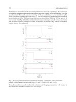
Example trajectory of the control system with the discretization step h =0.1
and the initial conditions y
(0)
=(1, 1, 0, 0, 0, 1.01)
T
isshowninFig.1.After
12 iterations the first change of symbol occurs, and from then on the symbols
alternate (see Fig. 1(b)).
The trajectory converges to the period–2 orbit
y

=(−0.03999998, −3.436·10
−7
, 6.872·10
−6
, −0.04013, 0.002624, −0.05249)
T
,
y

=(−0.04000002, 3.436·10
−7
, −6.872·10
−6

, −0.03987, −0.002624, 0.05249)
T
.
According to the Theorem 2 bounds for the steady state are
(0.0500000172, 3.436·10
−7
, 6.872·10
−6
, 0.050131, 0.002624, 0.05249)
T
.
132 Z. Galias and X. Yu
(a)
−0.5
0
0.5
1
1.5
2
−2
−1
0
1
−2
−1
0
1
2
x
1

x
2
x
3
(b)
−0.2
0
0.2
0.4
0.6
−0.4
−0.2
0
0.2
0.4
−1
−0.5
0
0.5
1
1.5
x
4
x
5
x
6
Fig. 1. Trajectory with the initial conditions y
(0)
=(1, 1, 0, 0, 0, 1.01)

T
converges to a
period–2 orbit
4 Conclusions
We have shown that the Euler’s discretization with appropriately chosen time
step is a good method for discrete implementation of SMC systems. We have
demonstrated that for the ECB-SMC systems with relative degree restriction, if
the discrete system is stable then every trajectory converges to a period–2 cycle.
We have found the bounds for the steady states and higher order sliding mode
functions, which allow us to estimate the maximum chattering amplitude when
using a given value of the time step.
It should be noted that there are some commonalities between the ECB-
SMC systems with relative degree higher than one, discretized by using the
Euler method and the results for continuous-time higher-order SMC systems
Euler’s Discretization of SMC Systems 133
[12, 13] where it was proved that, (if we use the same problem formula-
tion as in this chapter), for very small sampling period τ, |g
1
| <γ
1
τ
r+1
,
|g
i
| <γ
i
τ
r−i+1
, ···, |g

r+1
| <γ
r+1
τ, for some positive γ
1
, ···,γ
r
,γ
r+1
which
are qualitative bounds. In our results, the accurate bounds of steady states and
sliding mode functions have been given as shown in the Theorem 2.
Further work will be focused on the Euler’s discretization as well as the Zero-
Order-Hold sampling of the multi-input SMC systems.
References
1. Utkin, V.I.: Sliding Modes in Control Optimization. Springer, Berlin (1992)
2. Edwards, C., Spurgeon, S.: Sliding Mode Control: Theory and Applications. Taylor
and Francis, London (1998)
3. Sabanovic, A., Fridman, L.M., Spurgeon, S.: Variable Structure Systems: From
Principles to Implementation. IEE, London (2004)
4. Gao, W., Wang, Y., Homaifa, A.: Discrete-time variable structure control systems.
IEEE Transactions on Industrial Electronics 42, 117–122 (1995)
5. Yu, X., Chen, G.: Discretization behaviors of equivalent control based sliding-mode
control systems. IEEE Transactions on Automatic Control 48, 1641–1646 (2003)
6. Xia, X.H., Zinober, A.S.I.: Delta-modulated feedback in discretization of sliding
mode control. Automatica 42, 771–776 (2006)
7. Galias, Z., Yu, X.: Euler’s discretization of single input sliding mode control sys-
tems. IEEE Transactions on Automatic Control 52, 1726–1730 (2007)
8. Xu, J.X., Zheng, F., Lee, T.H.: On sampled data variable structure control sys-
tems. In: Young, K.K.D., Ozguner, U. (eds.) Variable Structure Systems, Sliding

Mode and Nonlinear Control. Lecture Notes in Control and Information Sciences,
vol. 274. Springer, New York (1999)
9. Misawa, E.A.: Discrete time sliding mode control: The linear case. ASME Journal
of Dynamic Systems Measurement and Control 119, 819–921 (1997)
10. Pan, Y., Furuta, K., Hatakeyama, S.: Invariant sliding sector for discrete time
variable structure control. In: Proc. 2000 Asian Control Conference, Shanghai,
China (2000)
11. Koshkouei, A.J., Zinober, A.S.I.: Sliding mode control of discrete–time systems.
ASME Journal of Dynamic Systems, Measurement, and Control 122, 793–802
(2000)
12. Fridman, L.M., Levant, A.: Higher order sliding modes. In: Sabanovic, A., Frid-
man, L.M., Spurgeon, S. (eds.) Variable Structure Systems: From Principles to
Implementation, IEE, London (2004)
13. Levant, A.: Higher order sliding modes, differentiation and output-feedback control.
International Journal of Control 76, 924–941 (2003)
14. Wang, B., Yu, X., Chen, G.: Discretization behaviors of sliding mode control sys-
tems with matched uncertainties. In: Proc. WCICA 2006, Dalian, China (2006)
15. Rubio, J.D., Yu, W.: A new discrete-time sliding mode control with time-varying
gain and neural identification. International Journal of Control 79, 338–348 (2006)