Tài liệu tiếng anh về backtracking
Bạn đang xem bản rút gọn của tài liệu. Xem và tải ngay bản đầy đủ của tài liệu tại đây (145.22 KB, 13 trang )
Chapter 3
Backtracking
3.1 Introduction
Backtracking is a very general technique that can be used to solve a wide variety of problems
in combinatorial enumeration. Many of the algorithms to be found in succeeding chapters
are backtracking in various guises. It also forms the basis for other useful techniques such
as branch-and-bound and alpha-beta pruning, which find wide application in operations
research (and, more generally, discrete optimization) and artificial intelligence, respectively.
As an introductory problem, consider the puzzle of trying to determine all way s to place
n non-taking queens on an n by n chessboard. Recall that, in the game of chess, the queen
attacks any piece that is in the same row, column or either diagonal. To gain insight, we
first consider the specific value of n = 4. We start with an empty chessboard and try to
build up our solution column by column, starting from the left. We can keep track of the
approaches that we explored so far by maintaining a backtracking tree whose root is the
empty board and where each level of the tree corresponds to a column on the board; i.e., to
the number of queens that have been places so far. Figure 3.1 shows the backtracking tree.
This tree is constructed as follows: Starting from an empty board, try to place a queen
in column one. There are four positions for the queen, which correspond to the four children
of the root. In column one, we first try the queen in row 1, then row 2, etc., from left to
right in the tree. After successfully placing a queen in some column we then proceed to the
next column and recursively try again. If we get stuck at some column k, then we backtrack
to the previous column k − 1, where we again try to advance the queen in column k − 1
from its current position. Observe that the tree is constructed in preorder. All nodes at
level n represent solutions; for n = 4 there are two solutions.
Let us consider now the case of a standard 8 by 8 chessboard. Here the problem is too
large to do the backtrack ing by hand, unless you are extremely patient. It is easier to write
a program.
The backtracking process, as described above, is recursive, so it is not surprising that
we can use a recursive procedure to solve the eight queens problem. A pseudo-Pascal
procedure for doing this is developed next. The solution x consists of a permutation of
1 through 8, representing the row locations of the queens in successive columns. For the
4-queens problem the permutations giving solutions were x = [2, 4, 1, 3] and x = [3, 1, 4, 2].
As the algorithm is proceeding we need some way to determine whether a queen is being
attacked by another queen. The easiest way to do this is to maintain three boolean arrays,
call them a, b, c. The array a indicates if a row does not contain a queen. The array
41
42 CHAPTER 3. BACKTRACKING
•
•
•
•
•
•
•
•
•
•
•
•
•
•
•
•
•
•
•
•
•
•
•
•
•
•
•
•
•
•
•
•
•
•
•
•
❅
❅
❅
❅
❅
❅✦
✦
✦
✦
✦
✦
✦
✦
❛
❛
❛
❛
❛
❛
❛
❛
Figure 3.1: The four queens backtracki ng tree.
b indicates if a diagonal does not contain a queen, and c indicates if a diagonal
does not contain a queen. The sum of the row and column indices is constant along
diagonals, and the difference of the row and column indices is constant along diagonals.
Thus a is indexed 1 8, array b is indexed 2 16, and c is indexed -7 7.
1
These arrays
are initialized to be true, and then we call Queen( 1 ). The solution is given in the global
array x, which need not be initialized.
(Q1) procedure Queen ( col : N )
(Q2) local row : N;
(Q3) for row := 1 to 8 do
(Q4) if a[row] and b[row+col] and c[row −col] then
(Q5) x[col ] := row;
(Q6) a[row ] := b[row+col ] := c[row −col ] := false;
(Q7) if col < 8 then Queen( col + 1 ) else PrintIt;
(Q8) a[row ] := b[row+col ] := c[row −col ] := true;
Algorithm 3.1: Algorithm for the 8 queens problem.
It turns out that there are 92 solutions to the 8 by 8 puzzle. Only 12 of the solutions
are non-isomorphic in the sense that all other solutions may be obtained from these 12 by
rotating and/or flipping the board.
1
In other languages, the indexing of c may have to be offset.
uvic01,
c
Frank Ruskey, 1995–2001
3.2. BACKTRACKING ALGORITHMS 43
3.2 Backtracking Algorithms
In the general backtracking scenario we wish to generate all strings S that satisfy some
predicate P.
S = {(x
1
x
2
x
3
· · ·) ∈ A
1
× A
2
× A
3
× · · · |P (x
1
x
2
x
3
· · ·)}
Each A
i
is a finite set. Of course, the strings must be of finite length and there must be
finitely many of them. In most applications the strings will have a fixed length. In order
to apply the backtracking technique the predicate P must be extended to a predicate Q
defined on “prefix” strings such that the following properties hold:
P (x
1
x
2
x
3
· · ·) implies Q(x
1
x
2
x
3
· · ·), and
¬Q(x
1
x
2
· · · x
k−1
) implies ¬Q(x
1
x
2
· · · x
k−1
x) for all x ∈ A
k
(3.1)
In other words, if a string does not satisfy the predicate Q then it cannot be extended
to a string that does satisfy the predicate P . Given a partial solution x = x
1
x
2
· · · x
k−1
we
let S
k
(x) denote all the valid ways of extending the string by one element. If the string x
is understood we simply write S
k
. In other words,
S
k
(x) = {x ∈ A
k
| Q(xx)}.
The vertices of the backtracking tree are all those strings that satisfy Q. The children of
a vertex are all those sequences obtained from the parent sequence by appending a single
element.
As an illustration of the preceeding definitions consider the 8 by 8 non-taking queens
problem. The sets A
i
are {1,2,. . . ,8} for each i = 1, 2, . . . ,8. The predicate Q is simply
whether the queens placed so far are non-taking. An example in which the sets A
i
differ
for different i will be given in the next section.
A recursive procedure for the general backtracking scenario is deceptively simple. It is
given in Algorithm 3.2. The initial call is Back(1, ε); no initialization is necessary. The call
Back(k, x) generates all strings of the form xy for which xy ∈ S.
The parameter x, representing a partial solution, is often left as a global variable, as
it was in our procedure for the 8 queens problem. Another property that the 8 queens
solutions have is that they are all strings of the same length. This is usually the case and
results in a simplification of the algorithm. Suppose that all solutions have length n. Then
Back can be modified by making lines (B5) and (B6) into the else cl ause of the if statement
at line (B4). If, in addition, Q(x
1
x
2
· · · x
n
) implies P (x
1
x
2
· · · x
n
), then the test for P (x) at
line (B4) can be replace by the test “k > n”. This is done in many of the procedures to be
found in succeeding chapters.
(B1) procedure Back ( k : N; x : string);
(B2) local x : A
k
; S
k
: set of A
k
(B3) begin
(B4) if P (x) then PrintSolution( x );
(B5) compute S
k
;
(B6) for x ∈ S
k
do Back( k + 1, xx );
(B7) end {of Back};
Algorithm 3.2: Recursive backtracking algorithm.
uvic01,
c
Frank Ruskey, 1995–2001
44 CHAPTER 3. BACKTRACKING
We also present a non-recursive version of the algorithm; see Algorithm 3.3. This version
is of interest when speed is of utmost concern — for example, if the backtracking routine is
being written in assembly language.
k := 1;
compute S
1
;
while k > 0 do
while S
k
= ∅ do
{Advance to next position}
x
k
:= an element of S
k
;
S
k
:= S
k
\ {x
k
};
if P (x
1
x
2
· · · x
k
) then PrintSolution;
k := k + 1;
compute S
k
;
{Backtrack to previous position}
k := k − 1;
end;
Algorithm 3.3: Non-recursive backtracking algorithm.
3.3 Solving Pentomino Problems with Backtracking.
As a somewhat more complicated problem we consider a pentomino problem. A pentomino
is an arrangement of five unit squares joined along their edges. They were popularized
by Golomb [169]
2
. There are 12 non-isomorphic pentominoes as shown in Figure 3.2.
The pieces have been given and arbritrary numbering; traditionally letters have also been
associated with the pieces and we show those as well. We will develop an algorithm to find
all ways of placing the 12 pentomino pieces into a 6 by 10 rectangle. It turns out that
there are 2,339 non-isomorphic ways to do this. One of the solutions is shown in Figure
3.3. Each piece can be rotated or flipped, which can give different orientations of a piece.
Piece 1 has 1 orientation, piece 2 has two orientations, pieces 3,4,5,6,7 have 4 orientations,
and pieces 8,9,10,11,12 have 8 orientations. Each solution to the problem is a member of an
equivalence class of 4 other solutions, obtained by flipping and rotating the 6 by 10 board.
Figure 3.4 shows how the board is numbered. It also shows a particular placement of
the “X” piece. This placement is represented by the set [8,13,14,15,20]. Every placement
of a piece is represented by some 5-set. The anchor of a placement is the smallest number
in the 5-set.
The backtracking algorithm successively tries to place a piece in the lowest numbered
unoccupied square; call it k. Once k is determined we try to place an unused piece over it.
The pieces are tried in the order 1, 2, . . . , 12 as numbered in Figure 3.2. Thus we wish to
know, for each piece and number k, all placements that are anchored at k. These placements
are precomputed and stored in the array List from the type and variable declarations of
Figure 3.4. For example, the placement of “X” in Figure 3.4 is the only set in List[1,8].
Of course, the list usually contains more than one element; List[12,8] has eight members,
2
The term pentomino, for a 5-omino, is a registered trademark of Solomon W. Golomb (No. 1008964,
U.S. Patent Office, April 15, 1975).
uvic01,
c
Frank Ruskey, 1995–2001
3.3. SOLVING PENTOMINO PROBLEMS WITH BACKTRACKING. 45
8 − N 9 − L
1 − X 3 − V 4 − U 5 − W 6 − T
10 − Y
2 − I
7 − Z 11 − F 12 − P
Figure 3.2: The 12 pentomino pieces.
Figure 3.3: A solution to the 6 by 10 pentomino problem.
00
1
2
3
4
5
6
7
8
9
10
11
12
13
14
15
16
17
18
19
20
21
22
23
24
25
26
27
28
29
30
31
32
33
34
35
36
37
38
39
40
41
42
43
44
45
46
47
48
49
50
51
52
53
54
55
56
57
58
59
Figure 3.4: Numbering the board (and the placement of a piece).
uvic01,
c
Frank Ruskey, 1995–2001
46 CHAPTER 3. BACKTRACKING
15
7 13
18
14
19 7
7
18
20
15
8
7
7
12
13
20
21
13
14
14
12
1913
12
7
820
13
12
14
14 20
7 13
7
59
0
Figure 3.5: Lists for piece 11, with those anchored at location 7 shown explicitly.
the maximum possible number. The list for List[11,7] is shown in Figure 3.5. Piece 7
has 8 orientations but only 7 of them appear on the list because one of them would extend
outside of the board. The one not appearing is blank in Figure 3.5. The others show the 5
numbers that are in the set correspoding to piece 11 anchored at position 7.
type
PieceNumber = Z(1 . . . 12);
BoardNumber = Z(0 . . . 63);
Board = word(BoardNumber);
ListPtr = pointer to ListElement;
ListElement = node(Position : Board,Link : ListPtr);
global
TheBoard : Board;
List : array [PieceNumber,BoardNumber] of Li stPtr;
PieceAvail : word(PieceNumber);
Solution : array[PieceNumber] of ListPtr;
Algorithm 3.4: Declarations for pentomino program.
With these global declarations the backtracking procedure is given in Figure 3.5. Inter-
section ( ∩ ) is used to determine whether a piece can be placed without overlap, union ( ∪
) is used to add a new piece to the board, and difference (\) is used to remove a piece from
the board. If the set operations are correctly implemented using AND, OR, and NOT on
machine words, then this program will be quite fast.
It is natural to wonder whether the backtracking can b e sped up by checking for isolated
squares. That is to say, checking whether the unused portion of the board has a number of
squares divisible by five before trying to place the next piece. This strategy will certainly
cut down on the number of vertices in the backtracking tree, but now more work is done
at each vertex. In the author’s experience it does not pay to check for isolated squares; the
extra work done at each vertex i s greater than the savings obtained by having a smaller
tree. Backtracking is full of such tradeoffs between the size of the tree and the amount of
work done at each vertex.
The more general question that this raises is: Among two predicates Q and R both
satisfying (3.1), which is better? Of course the ultimate test is in the running time of the
uvic01,
c
Frank Ruskey, 1995–2001
3.3. SOLVING PENTOMINO PROBLEMS WITH BACKTRACKING. 47
procedure BackTrack ( k : BoardNumber );
local pc : PieceNumber;
while k ∈ TheBoard do k := k + 1;
for pc := 1 to 12 do
if pc in PieceAvail then
PieceAvail := PieceAvail \ [pc];
Solution[pc] := List[pc,k];
while Solution[pc] = null do
if TheBoard ∩ Solution[pc].Position = ∅ then
TheBoard := TheBoard ∪ Solution[pc].Position;
if PieceAvail = ∅
then PrintSolution
else BackTrack( k + 1 );
TheBoard := TheBoard \ Solution[pc].Position;
Solution[pc] := Solution[pc].Link;
PieceAvail := PieceAvail ∪ [pc];
end {of BackTrack}
Algorithm 3.5: Backtracking routine for pentomino problem.
two algorithms that arise. Two extremes are worth noting. If Q is always true then (3.1) i s
satisfied. No pruning of the backtracking is done; all of A
1
× A
2
× · · · is generated. What
if Q is perfect? That is, what if Q(x) implies that there is some y such that P (xy)? Then
every leaf of the backtracking tree is in S. As mentioned in Chapter 1, this is the BEST
propery: Backtracking Ensuring Success at Terminals.
3.3.1 Eliminating Isomorphic Solutions
Reject isomorphs! The is no reason to generate isomorphic solutions when generating
all solutions to pentomino and other “space-filling” puzzles. In particular, for the 6 by
10 pentomino puzzle, each solution has four equivalent solutions (including itself) in the
equivalence class obtained by rotating and flipping. Thus, even if we wanted all solutions,
isomorphic or not, we could generate the non-isomorphic ones and then flip and rotate to
get the others. As we will see, there is absolutely no computational overhead in rejecting
isomorphic solutions in the 6 by 10 case, so that we save a factor of 4 in the running time.
In general, the basic idea is to fix the positions and orientations of some selected piece
(or pieces). Two properties are necessary: (a) Each equivalence class must have a member
with the selected piece in the one of the fixed positions and orientations, and (b) each
of the symmetries of the board must move the piece out of the set of fixed positions and
orientations.
For the 6 by 10 pentomino problem we will fix the center square of the “X” shaped piece
so that it lies in the upper quadrant (thinking of the board as being centered at its center).
See Figure 3.6.
uvic01,
c
Frank Ruskey, 1995–2001
48 CHAPTER 3. BACKTRACKING
Figure 3.6: Eliminating isomorphs in the 6 by 10 pentomino puzzle.
3.4 Estimating the Running Time of Backtracking.
In many instances it is useful to obtain an estimate of the number of vertices that will occur
in a backtracking tree, before the actual algorithm is run. The estimate presented in this
section only applies in those instances when we are searching for all possible solutions (i.e.
the entire tree is being examined).
The basic idea is to run an experiment in which we follow a random path in the tree
from the ro ot to a leaf, and then assume that the entire tree has a similar “parent” -
“number of children relationship” as the vertices on this path. The random path i s chosen
by successively picking a random child of the current vertex to be included next in the
path. Each child is regarded as being equally likely. For example, consider the tree shown
in Figure 3.7(a) where the thickened edges i ndicates the random path.
In the experiment the root had three children, the root’s child on the thickened path
had two children, and so on. Thus we assume that the root has three children, all children
of the root have two children, etc. This gives rise to the tree of Figure 3.7(b). This tree has
1 + 3 + 3 ·2 + 3 · 2 · 1 + 3 · 2· 1 · 2 + 3 · 2· 1· 2 · 1 = 40 vertices. In general, let n
k
denote the
degree of the (k − 1)st vertex along the experimental path. There are n
1
n
2
· · · n
k
vertices
at level k in the assumed tree. Thus the estimate is the (finite) sum
X = 1 + n
1
+ n
1
n
2
+ n
1
n
2
n
3
+ · · ·.
A procedure to compute the estimate is given in Algorithm 3.6. A recursive version can
also be easily derived.
For any probabilistic estimate a desirable property is that the exp ected value of the
estimate is equal to the quantity being estimated. In probability theory such an estimator
uvic01,
c
Frank Ruskey, 1995–2001
3.4. ESTIMATING THE RUNNING TIME OF BACKTRACKING. 49
Figure 3.7: (a) True backtracking tree with random root-to-leaf path shown. (b) Assumed
tree from that random path.
estimate := product := 1;
k := 1;
compute S
1
;
while S
k
= ∅ do
{Advance}
n
k
:= |S
k
|;
product := n
k
· product;
estimate := estimate + product;
x
k
:= an element of S
k
, chosen at random;
k := k + 1;
compute S
k
;
Algorithm 3.6: Estimation algorithm.
uvic01,
c
Frank Ruskey, 1995–2001
50 CHAPTER 3. BACKTRACKING
is referred to as being unbiased. Let T be the tree whose size |T| is being estimated.
Intuitively, the reason that the estimate is unbiased is that the probability of reaching a
vertex x in the tree whose ancestors have degrees n
1
, n
2
, . . . , n
t
is equal to 1/(n
1
n
2
· · · n
t
),
which is the inverse of the weight assigned to that vertex by X. We will now give a more
formal argument. Define two functions on the vertices v of the backtracking tree:
τ(v) =
1 if v is the root
deg(¯v) · τ(¯v) if v has parent ¯v
and
I(v) = [[vertex v is visited in the experiment]].
Recall the [[]] notation, defined the previous chapter: [[P ]] is 1 if P is true and is 0 if P is
false. Note that τ depends only on the tree and not the experiment. The random variable
X may be rewritten as
X =
v∈T
τ(v) · I(v).
Now take the expected value of the random variable X and use linearity of expectation to
obtain
E(X) =
v∈T
τ(v) · E(I(v)) =
v∈T
τ(v) ·
1
τ(v)
=
v∈T
1 = |T|.
The estimator is therefore unbiased.
Some care should be exercised in applying this estimate. Backtracking trees tend to
vary wildly in their structure and subtrees with many vertices may be well hidden in the
sense that they are accessed only through paths from the root with vertice s of low degree.
It is essential in applying the test that a large number of trials are used. Once this is done,
however, the test is remarkably effective.
3.5 Exercises.
1. [1+] Use backtracking by hand to determine the number of solutions to the 5 by 5
queens problem. How many of the solutions are non-isomorphic?
2. [1] Generate an estimate of the number of vertices in the backtracking tree for the 8
by 8 queens problem. In picking your “random” row positions, simply use the lowest
numbered valid row.
3. [1+] Show that the number of solutions to the n by n Queens problem is less than or
equal to n(n − 4) · (n − 2)!. Can you derive a better bound?
4. The following 150 characters of C code outputs the number of solutions to the n-
Queens problem. Explain how the code works. What’s the largest value of n for
which it will produce a correct answer (after a potentially very long wait) on your
machine?
uvic01,
c
Frank Ruskey, 1995–2001
3.5. EXERCISES. 51
Figure 3.8: The Soma cube pieces.
t(a,b,c){int d=0,e=a&~b&~c,f=1;if(a)for(f=0;d=(e&=~d)&-e;f+=t(a&~d,(b|d)<<1,
(c|d)>>1));return f;}main(q){scanf("%d",&q);printf("%d\n",t(~(~0<<q),0,0));}
5. [2] Write a backtracking program to determine a configuration containing the smallest
number of queens on a n by n b oard so that every square of the board is under attack.
Is the problem easier if the queens are specified to be non-taking? Give explicit
solutions for 1 ≤ n ≤ 8.
6. [1+] How many hexominoes (6-ominoes) are there? [2] Prove that the set of all
hexominoes cannot be placed in a rectangular configuration without holes.
7. [3−] Define the order of a polyomino to be the smallest number of copies of P that
will fit perfectly into a rectangle, where rotations and reflections of P are allowed.
The figure below shows that the pentomino
has order at most 10. Show that
its order is exactly 10. What are the orders of the other two polyomino shapes shown
below?
8. [2] A polyomino puzzle with the following pieces has been marketed.
The puzzle is to place the pieces on an 8 by 8 board. Write a backtracking program
to determine the number of different non-isomorphic solutions.
9. [2] The Soma Cube puzzle is to fit the seven pieces listed in Figure 3.8 into a 3 by 3
by 3 cube . Write a backtracking program to generate all 240 non-isomorphic solutions
to the Soma Cube puzzle.
10. [2] Snake-in-a-cube puzzle: A snake consists of 27 unit cubes arranged in order. They
are held together by a sho ck-cord, but can be rotated around the cord. Each unit cube
is either ”straight-through” (the cord passed through one face of the cube and exits
uvic01,
c
Frank Ruskey, 1995–2001
52 CHAPTER 3. BACKTRACKING
✈ ✈ ✈ ✈ ✈ ✈
✈ ✈ ✈ ✈ ✈ ✈
✈ ✈ ✈ ✈ ✈ ✈
✈ ✈ ✈ ✈ ✈ ✈
✈ ✈ ✈ ✈ ✈ ✈
✈ ✈ ✈ ✈ ✈ ✈
✁
✁
✁
✁
✁
✁
❆
❆
❆
❆
❆
❆
✟
✟
✟
✟
✟
✟
✟
✟
✟
✟
✟
✟
❍
❍
❍
❍
❍
❍
❍
❍
❍
❍
❍
❍
❆
❆
❆
❆
❆
❆
❍
❍
❍
❍
❍
❍
✟
✟
✟
✟
✟
✟
❆
❆
❆
❆
❆
❆
❆
❆
❆
❆
❆
❆
❆
❆
❆
❆
❆
❆
❍
❍
❍
❍
❍
❍
✁
✁
✁
✁
✁
✁
✟
✟
✟
✟
✟
✟
❆
❆
❆
❆
❆
❆
❆
❆
❆
❆
❆
❆
❆
❆
❆
❆
❆
❆
❍
❍
❍
❍
❍
❍
❆
❆
❆
❆
❆
❆
✁
✁
✁
✁
✁
✁
❆
❆
❆
❆
❆
❆
✁
✁
✁
✁
✁
✁
❍
❍
❍
❍
❍
❍
❆
❆
❆
❆
❆
❆
✟
✟
✟
✟
✟
✟
✁
✁
✁
✁
✁
✁
✟
✟
✟
✟
✟
✟
❍
❍
❍
❍
❍
❍
❍
❍
❍
❍
❍
❍
✟
✟
✟
✟
✟
✟
❍
❍
❍
❍
❍
❍
✁
✁
✁
✁
✁
✁
✁
✁
✁
✁
✁
✁
❍
❍
❍
❍
❍
❍
Figure 3.9: A 6 by 6 knight’s tour.
throught the opposite face) or is an ”elbow” (the cord passed through one face and
exists through another perpendicular face). The problem is to find all way of shaping
the snake into a 3x3x3 cube. A specific instance of the snake has been marketed and
has the following 27 cubes SSESESESEEEESESEEESEESEEESS, where S indicates
straight-through, and E indicates elbow. Determine the number of non-isomorphic
solutions of this puzzle, and of the puzzle where every unit cube is an elbow.
11. [2] A knight’s tour of an n by n chessboard is a sequence of moves of the knight on
the chessboard so that each of the n
2
squares is visited exactly once. Shown in Figure
3.9 is a knight’s tour of a 6 by 6 chessboard. Write a backtracking program to find
a single knight’s tour on an 8 by 8 chessboard starting from the upper left corner. A
knight’s tour that returns to the square upon which it started is said to be re-entrant.
Modify your program from so that it finds a re-entrant k night’s tour. Estimate the
time that it would take to explore the entire backtracking tree assuming that it takes
a millisecond to process one vertex in the tree. Prove that no Knight’s tour can exist
if n is odd.
12. [1+] Draw a graph representing the possible moves of a knight on a 4 by 4 chessboard.
Use this graph to prove that there is no knight’s tour on a 4 by 4 board.
13. [2] In a noncrossing Knight’s tour the lines drawn for each move of the knight do
not cross. The tour shown in Figure 3.9 has many crossings, and in general, a non-
crossing tour cannot visit every square of the board. Determine the longest possible
non-crossing knight’s tour on an 8 by 8 board.
14. [2] Write a backtracking program to determine the number of ways to color the vertices
of a graph with k colors for k = 1, 2, . . . , n where n is the number of vertices in the
graph. In any such coloring adjacent vertices must receive distinct colors. Deciding
whether a graph can be colored with k colors is a well-known NP-complete problem.
15. [2] Write a backtracking program to count the number of topological sortings (linear
extensions) of a directed acyclic graph (partially ordered set).
uvic01,
c
Frank Ruskey, 1995–2001
3.6. BIBLIOGRAPHIC REMARKS 53
16. [2] Write a backtracking program to list all Hamilton cycles (if any) in a graph. Use
your program to determine the number of Hamilton cycles in the tesseract.
17. [2] For given k, a subset K ⊆ [k], is said to represent k if there is some unique I ⊆ K
such that
x∈I
x = k. For given n, a pair of subsets P, Q ⊆ [n] is said to dichotomize
[n] if, for each k ∈ [n], the number k is representable by P or by Q, but not by
both. For example {1, 2, 6}, {4, 5} dichotomizes [9], but [12] is not dichotomized by
{1, 2, 9}, {3, 4, 5} since 3 and 9 are represented twice and 6 is not represented. Write
a backtracking program that takes as input n and outputs all pairs of subsets of [n]
that dichotomize it. How many solutions are there for n = 17?
18. [3] Let τ = (1 2) and σ = (1 2 · ·· n). Write a backtracking program to find a
Hamilton cycle in the directed Cayley graph Cay(S
n
: {σ, τ}) when n = 5. Can you
find a Hamilton path for n = 6? [R−] Find a Hamilton cycle for n = 7. It is known
that there is no Hamilton cycle for n = 6.
19. There is a large family of combinatorial questions involving the packing of squares
into squares. [2+] For n ≤ 13 determine the least number of smaller squares that will
tile a n by n square. [2+] The sum 1
2
+ 2
2
+ · · · + 24
2
= 70
2
suggests that it might
be possible to tile a 70 by 70 square with squares of sizes 1, 2, . . . , 24. Show that this
is impossible.
20. [1] Write Algorithm 3. 6 as a recursive procedure.
21. [3] Extend the unbiased procedure for estimating the size of a backtracking tree to
that of estimating the size of a directed acyclic graph that is rooted at r (all vertices
are reachable from r).
3.6 Bibliographic Remarks
Perhaps the first description of the general backtrack ing technique is in Walker [474]. Early
papers about backtracking include Golomb and Baumert [171].
The eight queens problem is attributed to Nauck (1850) by Schuh [409]. It is said that
Gauss worked on the problem and obtained the wrong answer! Sosic and Gu [430] analyze
programs for the 8-queens problem.
A paper of Bitner and Re ingold [43] discusses a number of interesting ways to speed up
backtracking programs and contains some applications to polyomino problems.
A (very ugly) program for generating all solutions to the Soma cube problem may be
found in Peter-Orth [335].
The book that really popularized polyominoes, and pentominoes in particular, is “Poly-
ominoes” by Golomb [169]. The book by Martin [290] contains much interesting material
about polyominoes and contains further references on the topic. The two volume book
by Berlekamp, Conway and Guy [38] on mathematical games contains interesting chapters
about the Soma cube (including a map of all solutions!) as well as scattered references to
polyominoes.
The method for estimating the size of the backtracking tree comes from Hall and Knuth
[184] and further analysis is carried out in Knuth [240]. The efficiency of the method has
been improved by Purdom [353]. The estimation method can be extended from rooted trees
to directed acyclic graphs; see Pitt [340].
uvic01,
c
Frank Ruskey, 1995–2001