Đề thi Olympic quốc tế 2013 - Bài 3 môn vật lý
Bạn đang xem bản rút gọn của tài liệu. Xem và tải ngay bản đầy đủ của tài liệu tại đây (726.49 KB, 4 trang )
The Greenlandic Ice Sheet
T3
Page 1 of 4
Introduction
This problem deals with the physics of the Greenlandic ice sheet, the second largest glacier in the
world, Fig. 3.1(a). As an idealization, Greenland is modeled as a rectangular island of width and
length with the ground at sea level and completely covered by incompressible ice (constant
density
), see Fig. 3.1(b). The height profile of the ice sheet does not depend on the -
coordinate and it increases from zero at the coasts to a maximum height
along the
middle north-south axis (the -axis), known as the ice divide, see Fig. 3.1(c).
(c)
Figure 3.1 (a) A map of Greenland showing the extent of the ice sheet (white), the ice-free, coastal regions
(green), and the surrounding ocean (blue). (b) The crude model of the Greenlandic ice sheet as covering a
rectangular area in the -plane with side lengths and . The ice divide, the line of maximum ice sheet
height
runs along the -axis. (c) A vertical cut (-plane) through the ice sheet showing the height
profile (blue line). is independent of the -coordinate for , while it drops abruptly
to zero at and . The -axis marks the position of the ice divide. For clarity, the vertical
dimensions are expanded compared to the horizontal dimensions. The density
of ice is constant.
The Greenlandic Ice Sheet
T3
Page 2 of 4
Two useful formulas
In this problem you can make use of the integral:
and the approximation
, valid for
.
The height profile of the ice sheet
On short time scales the glacier is an incompressible hydrostatic system with fixed height profile
.
3.1
Write down an expression for the pressure inside the ice sheet as a function of
vertical height z above the ground and distance from the ice divide. Neglect the
atmospheric pressure.
0.3
Consider a given vertical slab of the ice sheet in equilibrium, covering a small horizontal base area
between and , see the red dashed lines in Fig. 3.1(c). The size of does not matter.
The net horizontal force component on the two vertical sides of the slab, arising from the
difference in height on the center-side versus the coastal-side of the slab, is balanced by a friction
force
from the ground on the base area , where
.
3.2a
For a given value of , show that in the limit ,
, and determine k
0.9
3.2b
Determine an expression for the height profile
in terms of
, ,,
and
distance from the divide. The result will show, that the maximum glacier height
scales with the half-width as
.
0.8
3.2c
Determine the exponent with which the total volume
of the ice sheet scales with
the area of the rectangular island,
.
0.5
A dynamical ice sheet
On longer time scale, the ice is a viscous incompressible fluid, which by gravity flows from the
center part to the coast. In this model, the ice maintains its height profile in a steady state,
where accumulation of ice due to snow fall in the central region is balanced by melting at the coast.
In addition to the ice sheet geometry of Fig. 3.1(b) and (c) make the following model assumptions:
1) Ice flows in the -plane away from the ice divide (the -axis).
2) The accumulation rate (m/year) in the central region is a constant.
3) Ice can only leave the glacier by melting near the coasts at .
4) The horizontal (-)component
of the ice-flow velocity is independent of .
5) The vertical -)component
of the ice-flow velocity is independent of .
Consider only the central region close to the middle of the ice sheet, where height
variations of the ice sheet are very small and can be neglected altogether, i.e.
.
3.3
Use mass conservation to find an expression for the horizontal ice-flow velocity
in terms of , , and
.
0.6
The Greenlandic Ice Sheet
T3
Page 3 of 4
From the assumption of incompressibility, i.e. the constant density
of the ice, it follows that
mass conservation implies the following restriction on the ice flow velocity components
3.4
Write down an expression for the dependence of the vertical component
of the
ice-flow velocity.
0.6
A small ice particle with the initial surface position
will, as time passes, flow as part of the
ice sheet along a flow trajectory in the vertical -plane.
3.5
Derive an expression for such a flow trajectory .
0.9
Age and climate indicators in the dynamical ice sheet
Based on the ice-flow velocity components
and
, one can estimate the age of the
ice in a specific depth
from the surface of the ice sheet.
3.6
Find an expression for the age of the ice as a function of height above ground,
right at the ice divide .
1.0
An ice core drilled in the interior of the Greenland ice sheet will penetrate through layers of snow
from the past, and the ice core can be analyzed to reveal past climate changes. One of the best
indicators is the so-called
, defined as
where
denotes the relative abundance of the two stable isotopes
and
of
oxygen. The reference
is based on the isotopic composition of the oceans around Equator.
Figure 3.2 (a) Observed relationship between
in snow versus the mean annual surface temperature .
(b) Measurements of
versus depth
from the surface, taken from an ice core drilled from surface
to bedrock at a specific place along the Greenlandic ice divide where
m.
The Greenlandic Ice Sheet
T3
Page 4 of 4
Observations from the Greenland ice sheet show that
in the snow varies approximately
linearly with temperature, Fig. 3.2(a). Assuming that this has always been the case,
retrieved
from an ice core at depth
leads to an estimate of the temperature near Greenland at the
age
.
Measurements of
in a 3060 m long Greenlandic ice core show an abrupt change in
at a
depth of 1492 m, Fig. 3.2(b), marking the end of the last ice age. The ice age began 120,000 years
ago, corresponding to a depth of 3040 m, and the current interglacial age began 11,700 years ago,
corresponding to a depth of 1492 m. Assume that these two periods can be described by two
different accumulation rates,
(ice age) and
(interglacial age), respectively. You can assume
to be constant throughout these 120,000 years.
3.7a
Determine the accumulation rates
and
.
0.8
3.7b
Use the data in Fig. 3.2 to find the temperature change at the transition from the ice age
to the interglacial age.
0.2
Sea level rise from melting of the Greenland ice sheet
A complete melting of the Greenlandic ice sheet will cause a sea level rise in the global ocean. As a
crude estimate of this sea level rise, one may simply consider a uniform rise throughout a global
ocean with constant area
.
3.8
Calculate the average global sea level rise, which would result from a complete melting
of the Greenlandic ice sheet, given its present area of
and
.
0.6
The massive Greenland ice sheet exerts a gravitational pull on the surrounding ocean. If the ice
sheet melts, this local high tide is lost and the sea level will drop close to Greenland, an effect
which partially counteracts the sea level rise calculated above.
To estimate the magnitude of this gravitational pull on the water, the Greenlandic ice sheet is now
modeled as a point mass located at the ground level and having the total mass of the Greenlandic ice
sheet. Copenhagen lies at a distance of 3500 km along the Earth surface from the center of the point
mass. One may consider the Earth, without the point mass, to be spherically symmetric and having
a global ocean spread out over the entire surface of the Earth of area
. All
effects of rotation of the Earth may be neglected.
3.9
Within this model, determine the difference
between sea levels in
Copenhagen (
) and diametrically opposite to Greenland (
).
1.8