An Efficient Tree-based Frequent Temporal Inter-object Pattern Mining Approach in Time Series Databases

VNU Journal of Science: Comp. Science & Com. Eng., Vol. 31, No. 1 (2015) 1-21

An Efficient Tree-based Frequent Temporal Inter-object
Pattern Mining Approach in Time Series Databases
Nguyen Thanh Vu, Vo Thi Ngoc Chau
*

Ho Chi Minh City University of Technology, Ho Chi Minh City, Vietnam


Abstract
In order to make the most of time series present in many various application domains such as finance, medicine,
geology, meteorology, etc., mining time series is performed for useful information and hidden knowledge.
Discovered knowledge is very significant to help users such as data analysts and managers get fascinating
insights into important temporal relationships of objects/phenomena along time. Unfortunately, two main
challenges exist with frequent pattern mining in time series databases. The first challenge is the combinatorial
explosion of too many possible combinations for frequent patterns with their detailed descriptions, and the
second one is to determine frequent patterns truly meaningful and relevant to the users. In this paper, we propose
a tree-based frequent temporal inter-object pattern mining algorithm to cope with these two challenges in a level-
wise bottom-up approach. In comparison with the existing works, our proposed algorithm is more effective and
efficient for frequent temporal inter-object patterns which are more informative with explicit and exact temporal
information automatically discovered from a time series database. As shown in the experiments on real financial
time series, our work has reduced many invalid combinations for frequent patterns and also avoided many
irrelevant frequent patterns returned to the users.
© 2015 Published by VNU Journal of Science.
Manuscript communication: received 15 December 2013, revised 06 December 2014, accepted 19 January 2015

Corresponding author: Vo Thi Ngoc Chau,

Keywords: Frequent Temporal Inter-Object Pattern, Temporal Pattern Tree, Temporal Pattern Mining, Support
Count, Time Series Mining, Time Series Rule Mining.

1. Introduction
An increasing popularity of time series
nowadays exists in many domains such as
finance, medicine, geology, meteorology, etc.
The resulting time series databases possess
knowledge that might be useful and valuable
for users to get more understanding about
behavioral activities and changes of the objects
and phenomena of interest. Thus, time series
mining is an important task. Indeed, it is the
third challenging problem, one of the ten
challenging problems in data mining research
pointed out in [30]. In addition, [10] has shown
this research area has been very active so far.
Among time series mining tasks, rule mining is
a meaningful but tough mining task shown in
[25]. This task is performed with a process
mainly including two main phases: mining
frequent temporal patterns and deriving
temporal rules representing temporal
associations between those patterns. In this
paper, our work focuses on the first phase for
frequent temporal patterns.
N.T. Vu et al. / VNU Journal of Science: Comp. Science & Com. Eng., Vol. 31, No. 1 (2015) 1-21

2

At present, we are aware of many existing
works related to the frequent temporal pattern
mining task on time series. Some that can be
listed are [3, 4, 5, 9, 14, 15, 16, 18, 19, 20, 26,
27, 29]. Firstly in an overall view about these
related works, it is realized that patterns are
often different from work to work and
discovered from many various time series
datasets. In a few works, the sizes and shapes of
patterns are fixed, and time gaps in patterns are
pre-specified by users. In contrast, our work
would like to discover patterns of interest that
can be of any shapes with any sizes and with
any time gaps able to be automatically derived
from time series. Secondly, there is neither data
benchmarking nor standardized definition of the
frequent temporal pattern mining problem on
time series. Indeed, whenever we get a mention
of frequent pattern mining, market basket
analysis appears to be a marvelous example of
the traditional association rule mining problem.
Such an example is not available in the time
series mining research area for frequent
temporal patterns. Thirdly, two main challenges
that need to be resolved for frequent pattern
mining in time series databases include the
problem of combinatorial explosion of too
many possible combinations for frequent

patterns with their detailed descriptions and the
problem of discovering frequent patterns truly
meaningful and relevant to the users.
Based on the aforementioned motivations,
we propose a tree-based frequent temporal
inter-object pattern mining algorithm in a level-
wise bottom-up approach as an extended
version of the tree-based algorithm in [20]. The
first extension is a generalized frequent
temporal pattern mining process on time series
databases with an adapted frequent temporal
pattern template. As a result, a frequent
temporal pattern in our work is semantics-based
temporal pattern that occurs as often as or more
often than expectation from users determined
by a minimum support count value. These
semantics-based temporal patterns are
semantically abstracted from one or many
different time series, each of which corresponds
to a time-ordered sequence of some repeating
behavioral activities of some objects or
phenomena of interest whose characteristic has
been observed and recorded over the time in its
respective time series. It is also necessary to
distinguish our so-called frequent temporal
patterns from motifs which are repeating
continuous subsequences in an individual time
series. In contrast, a frequent temporal pattern
being considered might contain various
repeating meaningful continuous subsequences

with many different temporal relationships
automatically discovered from one or many
different time series in the time series database.
As for the second extension, we have
reconsidered our tree-based algorithm
employing appropriate data structures such as
tree and hash table. The modified version of
this algorithm is defined with a keen sense of
reducing the number of invalid combinations
generated and checked for frequent temporal
patterns. It is also capable of removing many
irrelevant frequent patterns for the users.
As shown in the experiments on real
financial time series, our proposed algorithm is
more efficient to deal with the combinatorial
explosion problem. In comparison with the
existing works, our work is useful for frequent
temporal inter-object patterns more informative
with explicit and exact temporal information
which is automatically discovered from a time
series database.
The rest of our paper is structured as
follows. Section II provides an overall view of
the related works to point out the differences
between those works and ours. In section III,
we introduce a generalized frequent temporal
pattern mining process on time series databases
where our proposed algorithm is included. In
N.T. Vu et al. / VNU Journal of Science: Comp. Science & Com. Eng., Vol. 31, No. 1 (2015) 1-21
3

section IV, we propose an efficient tree-based
frequent temporal inter-object pattern mining
algorithm and its evaluation with many
experiments is presented and discussed in
section V. Finally, section VI concludes our
work and states several future works.
2. Related Works
In this section, some related works [3-7, 9,
14-22, 24, 26-29] are examined in comparison
with our work. Among these related works, [3-
5, 7, 9, 14-16, 18-20, 22, 26, 27] are proposed
for frequent temporal pattern mining in time
series, [21, 24, 29] for frequent sequential
pattern mining in sequential databases, and [6,
17, 28] for frequent temporal pattern mining in
temporal databases.
In the most basic form, motifs can be
considered as primitive patterns in time series
mining. There exist many approaches to find
motifs in time series named a few as [9, 15, 16,
19, 26, 27]. Our work is different from those
because the scope of our algorithms does not
include the phase of finding primitive patterns
that might be concerned with a motif discovery
algorithm. We suppose that those primitive
patterns are available to our proposed
algorithm. As for more complex patterns, [4]
has introduced a notion of perception-based
pattern in time series mining with a so-called

methodology of computing with words and
perceptions. [4] reviewed in details such
descriptions using sign of derivatives, scaling of
trends and shapes, linguistic interpretation of
patterns from clustering, a pattern generation
grammar, and temporal relationships between
patterns. Also towards perception-based time
series mining, [14] presented a duration-based
linguistic trend summarization of time series
using a few features such as the slope of the
line, the fairness of the approximation of the
original data points by line segments and the
length of a period of time comprising the trend.
Differently, our work concentrates on
discovering relationships among primitive
patterns. It is worth noting that our proposed
algorithms are not constrained by the number of
pattern types as well as the meanings and
shapes of primitive patterns. Moreover, [3] has
recently focused on discovering recent temporal
patterns from interval-based sequences of
temporal abstractions with two temporal
relationships: before and co-occur. Mining
recent temporal patterns in [3] is one step in
learning a classification model for event
detection problems. Different from [3], our
work belongs to the time series rule mining
task. Indeed, we would like to discover more
complex frequent temporal patterns in many
different time series with more temporal

relationships. For more applications, such
patterns can be used in other time series mining
tasks such as clustering, classification, and
prediction in time series. Based on the temporal
concepts of duration, coincidence, and partial
order in interval time series, [18] defined
pattern types from multivariate time series as
Tone, Chord, and Phrase. Tones representing
durations are labeled time intervals, which are
basic primitives. Chords representing
coincidence are formed by simultaneously
occurring Tones. Phrases are formed by several
Chords connected with a partial order which is
actually the temporal relationship “before” in
Allen’s terms. Support is used as a measure to
evaluate discovered patterns. As compared to
[18], our work supports more temporal
relationships with time information able to be
automatically discovered along with frequent
temporal inter-object patterns. Not directly
proposed for frequent temporal patterns in time
series, [22] made use of Allen’s temporal
relationships (before, equal, meets, overlaps,
during, starts, finishes, etc.) in their so-called
N.T. Vu et al. / VNU Journal of Science: Comp. Science & Com. Eng., Vol. 31, No. 1 (2015) 1-21

4

temporal abstractions. A temporal abstraction is
simply a description of a (set of) time series

through sequences of temporal intervals
corresponding to relevant patterns (i.e.
behaviors or properties) detected in their time
courses. These temporal abstractions can be
combined together to form more complex
temporal abstractions also using Allen’s
temporal relationships BEFORE, MEETS,
OVERLAPS, FINISHED BY, EQUALS, and
STARTS. It is realized that temporal
abstractions discovered from [22] are temporal
patterns rather similar to our frequent temporal
inter-object patterns. However, our work
supports richer trend-based patterns and also
provides a new efficient pattern mining
algorithm as compared to [22]. For another
form of patterns, [7] aimed to capture the
similarities among stock market time series
such that their sequence-subsequence
relationships are preserved. In particular, [7]
identified patterns representing collections of
contiguous subsequences which shared the
same shape for specific time intervals. Their
patterns show pairwise similarities among
sequences, called timing patterns using
temporal relationships such as begin earlier, end
later, and are longer. [7] also defined Support
Count and Confidence measures for a
relationship but these measures were not
employed in any algorithms of their work. As
compared to [7], our work supports more

temporal relationships with explicit time. More
recently, [5] has paid attention to linguistic
association rules in time series which are based
on fuzzy itemsets stemming from continuous
subsequences in time series. Each frequent
itemset in [5] can be considered as a frequent
pattern discovered in time series. However,
there is no consideration for temporal
knowledge in their frequent fuzzy itemsets. As
for [20], our work is based on their proposed
work with several extensions to the process and
tree-based algorithm in order to discover
frequent temporal inter-object patterns in a time
series database more efficiently.
In sequential database mining, [21, 24, 29]
are among many existing works on frequent
sequential pattern mining. [24] introduced GSP
algorithm to discover generalized sequential
patterns in a sequential database using Apriori
antimonotonic constraint. Later, [21] proposed
PrefixSpan algorithm to avoid the weakness of
[24] in scanning the database many times
unnecessarily. Indeed, [21] can find frequent
sequential patterns without generating any
candidate for them. For a comparison, those
frequent sequential patterns are not as rich as
ours in temporal aspects hidden in time series
which include interval-based relationships and
their associated time. As for [29], so-called
inter-sequence patterns are discovered with two

proposed algorithms which are M-Apriori and
EISP-Miner. The first algorithm is Apriori-like
and not as efficient as the second one which is
based on a tree data structure, named ISP-tree.
Nevertheless, the capability of both algorithms
is limited to a user-specified parameter which is
maximum span, called maxspan. It is believed
that it is not easy for users to provide a suitable
value for this parameter as soon as their
sequential database is mined. This might lead to
many trial-and-error experiments for maxspan.
In temporal database mining, [6, 17, 28]
worked for inter-transaction/inter-object
patterns/rules which involved one or many
different transactions/objects. Similarly, our
discovered frequent temporal patterns are inter-
object patterns. Differently, our patterns are
mined in the context of time series mining
where each component in our patterns is trend-
based with more degrees in change than
“up/down” or “increasing/decreasing” and
N.T. Vu et al. / VNU Journal of Science: Comp. Science & Com. Eng., Vol. 31, No. 1 (2015) 1-21
5

temporal relationships automatically derived are
interval-based with more time information than
point-based relationships “co-
occur/before/after”.
To the best of our knowledge, the type of
frequent temporal inter-object patterns defined

in our work has not yet been taken into
consideration in the existing works. The
proposed temporal frequent inter-object pattern
mining algorithm on a set of various time series
is designed to be a more efficient version of the
tree-based algorithm in [20].
3. A Generalized Frequent Temporal Inter-
object Pattern Mining Process
In this section, a generalized frequent
temporal inter-object pattern mining process on
a time series database is figured out to elaborate
our solution to discovering so-called frequent
temporal inter-object patterns from a given set
of different time series. This process is mainly
based on the one in [20]. Each time series is
considered an object of interest which can be
some phenomena or some physical objects in
our real life. We refer to a notion of temporal
inter-object pattern as temporal relationship
among objects being considered. This notion of
“inter-object” is somewhat similar to “inter-
transaction” in [17, 28] and “inter-sequence” in
[29]. However, our work aims to capture more
temporal aspects of their relationships so that
discovered patterns can be more informative
and applicable to decision making support. In
addition, interestingness of discovered patterns
is measured by means of the degree to which
they are frequent in the lifespan of these objects
in regard to a user-specified minimum threshold

called min_sup. This is because we use Support
Count as an objective measure with the
meaning intact in [12].
Depicted in Figure 1, the detail about the
pattern mining process will be mentioned
clearly as follows. Our process includes three
phases mainly based on the well-accepted
general knowledge discovery process [12].
Phase 1 is responsible for preprocessing to
prepare for semantics-based time series, phase 2
for the first step to obtain a set of repeating
trend-based subsequences, and phase 3 for the
primary step to fully discover frequent temporal
inter-object patterns. As compared to the
process in [20], our generalized process is not
specific for the input of the proposed algorithm
by relaxing the use of trend-based time series.
Instead, so-called semantics-based symbolic
time series are used so that users can have more
freedom to express the meaning of each
component in a resulting frequent pattern via
the semantic symbols used for time series
transformation in phase 1.
3.1. Phase 1 for Semantics-based Symbolic
Time Series
The input of this phase is also the one of
our work, which consists of a set of raw time
series of the same length for simplicity.
Formally, each time series TS is defined as TS
= (v

1
, v
2
, …, v
n
). TS is a so-called univariate
time series in an n-dimension space. The length
of TS is n. v
1
, v
2
, …, and v
n
are time-ordered
real numbers. Indices 1, 2, …, n correspond to
points in time in our real world on a regular
basis. Regarding semantics, time series is
understood as the recording of a quantitative
characteristic of an object or phenomenon of
interest observed regularly over the time.
G

N.T. Vu et al. / VNU Journal of Science: Comp. Science & Com. Eng., Vol. 31, No. 1 (2015) 1-21

6


Figure 1. A generalized frequent temporal inter-object pattern mining process on a time series database.
As previously mentioned, we have
generalized the pattern mining process

introduced in [20] for more semantics in
resulting frequent patterns. Thus, in this paper,
we do not restrict the meaning of individual
components in discovered frequent patterns to
behavioral changes of objects and the degree to
which they change. Instead, we enable so-called
semantics-based symbolic time series by means
of any transformation technique on time series.
For instance, each time series can be
transformed into a trend-based time series using
short-term and long-term moving averages in
[31] or into a symbolic time series using SAX
technique in [16].
The output of this phase is a set of
semantics-based time series each of which is
formally defined as (s
1
, s
2
, …, s
n
) where s
i
∈Σ
for i = 1 n where Σ is a discrete set of semantic
symbols derived by a corresponding
transformation technique. For the technique in
[31], Σ = {A, B, C, D, E, F} where A represents
the time series in a weak increasing trend; B in
a strong increasing trend; C starting a strong

increasing trend; D starting a weak increasing
trend; E in a strong decreasing trend; and F in a
weak decreasing trend. For the technique in
[16], Σ is the word book. If two breakpoints are
used, Σ = {a, b, c} where a represents
subsequences with high values, b with average
values, and c with low values.
3.2. Phase 2 for Repeating Subsequences
The input of phase 2 is exactly the output of
phase 1 which consists of one or many
semantics-based symbolic time series. The
main objective of phase 2 is to find repeating
subsequences in the input symbolic time series.
Such subsequences are indeed motifs hidden in
these time series. Regarding semantics, motifs
themselves are frequent parts in time series. As
compared to discrete point-based events in [17,
28], motifs in our work are suitable for the
applications where the time spans of an event
are significant to user’s problems. For example,
it is more informative for us to know that a
stock keeps strongly increasing three
consecutive days denoted by BBB from
Monday to Wednesday in comparison with a
simple fact such that a stock increases. As of
this moment, there are different approaches to
the motif discovery task on time series as
proposed in [9, 15, 16, 19, 26, 27]. This task is
out of the scope of our work. In our work, we
implemented a simple brute force algorithm to

extract repeating subsequences which are
motifs along with their counts, each of which is
the number of occurrences of the subsequence
in its corresponding symbolic time series.
Because of our interest in frequent patterns, we
consider repeating subsequences with at least
two occurrences. In short, the output of this
phase is a set of repeating subsequences with at
least two occurrences that might stem from
different objects.
N.T. Vu et al. / VNU Journal of Science: Comp. Science & Com. Eng., Vol. 31, No. 1 (2015) 1-21
7

3.3. Phase 3 for Frequent Temporal Inter-
object Patterns
Similar to phase 2, phase 3 has the input
which is the output of the previous phase, a set
of repeating subsequences. In addition, phase 3
also needs a minimum support count threshold,
min_sup, from users to evaluate the output
returned to users. As compared to [29], min_sup
is a single parameter whose value is provided
by the users along with the input set of time
series in our process. Using min_sup and the
input, phase 3 first obtains a set of primitive
patterns, named L
1
, which includes only
repeating subsequences with the counts equal or
greater than min_sup. All elements in L

1
are
called frequent temporal inter-object patterns at
level 1. At this level, there is just one object
involved in each frequent pattern. Differently,
level is used to refer to the number of
components in a pattern which will be detailed
below, not to the number of objects involved in
a pattern. Secondly, phase 3 proceeds with a
frequent temporal inter-object pattern mining
algorithm to discover and return to users a full
set of frequent temporal inter-object patterns in
a set of various time series. The rest of this
subsection will define a notion of frequent
temporal inter-object pattern and in section 4,
we will propose an extended version of the tree-
based frequent temporal inter-object pattern
mining algorithm that makes the frequent
temporal inter-object pattern mining process
more effective and efficient.
In general, we formally define a frequent
temporal inter-object pattern at level k for k>1
in the following form: m
1
-m
1
.ID<operator
type
1
: delta time

1
> m
2
-m
2
.ID….m
k-1
-m
k-1
.ID<
operator type
k-1
: delta time
k-1
> m
k
-m
k
.ID.
In this form, m
1
, m
2
, …, m
k-1
, and m
k
are
primitive patterns in L
1

which might come from
different objects whose identifiers are m
1
.ID,
m
2
.ID, …, m
k-1
.ID, and m
k
.ID, respectively.
Regarding relationships between the
components of a pattern at level k, operator
type
1
, …, operator type
k-1
are Allen’s temporal
operators. There are thirteen Allen’s temporal
operators in [1] well-known to express interval-
based relationships along the time, including
precedes (p), meets (m), overlaps (o), Finished
by (F), contains (D), starts (s), equals (e),
Started (S), during (d), finishes (f), overlapped
by (O), met by (M), preceded by (P). For their
converse relationships, our work used seven
Allen’s temporal operators (p, m, o, F, D, s, e)
to capture temporal associations between
subsequences from different objects in phase 3.
That is, operator type

1
, …, operator type
k-1
are
in {p, m, o, F, D, s, e}. Moreover, we use delta
time
1
, …, delta time
k-1
to keep time information
of the corresponding relationships. Regarding
semantics, intuitively speaking, a frequent
temporal inter-object pattern at level k for k>1
fully presents the relationships between the
frequent parts of different objects of interest
over the time. Hence, we believe that unlike
some other related works [7, 11, 17, 18], our
patterns are in a richer and more understandable
form and in addition, our pattern mining
algorithm is enabled to automatically discover
all such frequent temporal inter-object patterns
with no limitation on their relationship types
and time information.
Example 1: Let us consider a frequent
temporal pattern on a single object NY using
the transformation technique in [31]: AA-
NY<p:5>BBB-NY {0, 10, 20}. This pattern
enables us to know that after in a two-day weak
increasing trend, NY has a three-day strong
increasing trend and this fact repeats three times

at positions 0, 10, and 20 in the lifetime of NY.
Its illustration is given in Figure 2.
N.T. Vu et al. / VNU Journal of Science: Comp. Science & Com. Eng., Vol. 31, No. 1 (2015) 1-21

8


Figure 2. Illustration of a frequent temporal
pattern on a single object NY.



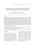
Figure 3. Illustration of a frequent temporal
inter-object pattern on two objects: NY and SH.
Example 2: Let us consider a frequent
temporal inter-object pattern on two objects NY
and SH also using the transformation technique
in [31]: AA-NY<e:2>AA-SH {0, 10}. This
pattern, whose illustration is presented in Figure
3, involves two objects NY and SH and
presents their temporal relationship along the
time. In particular, we can state about NY and
SH that NY has a two-day weak increasing
trend and in the same duration of time, SH does
too. This fact occurs twice at positions 0 and 10
in their lifetime. It is also worth noting that we
absolutely do not know whether or not NY
influences SH or vice versa in real life unless
their relationships are analyzed in some depth.
Nonetheless, such patterns provide us with

objective data-driven evidence on the
relationships among objects of interest so that
we can make other further thorough
investigations into these objects and their
surrounding environment.
4. The Proposed Tree-based Frequent
Temporal Inter-object Pattern Mining
Algorithm on Time Series Databases
As noted in [20], the type of knowledge we
aim to discover from time series has not yet
been considered. Hence, in [20], two mining
algorithms were defined: brute-force and tree-
based. The brute-force algorithm provides a
baseline for correctness checking and the tree-
based one helps speeding up the pattern mining
process in the spirit of FP-Growth algorithm
[13]. The two algorithms followed the level-
wise bottom-up approach.
Based on [20], we extend the tree-based
algorithm to a new version that enables us to
deal with the combinatorial explosion problem
by using an additional hash table for a detection
and elimination of irrelevant frequent patterns.
In particular, the modified tree-based algorithm is
capable of removing the instances of potential
candidates pertaining to one single pattern with
overlapping parts. In the following subsections,
the tree-based algorithm is detailed.
4.1. A Temporal Pattern Tree
In this paper, we remain a so-called

temporal pattern tree in [20]. Nevertheless, for
being self-contained, the description of a
temporal pattern tree is presented as follows.

Figure 4. The structure of a node in the temporal
pattern tree.

A temporal pattern tree (TP-tree) is a tree
that has n nodes of the same structure as shown
in Figure 4.
A node structure of a node being considered
in TP-tree is composed of the following fields:
- ParentNode: a pointer that points to a
parent node of the current node.
- OperatorType: an Allen’s temporal
operator in the form of <p>, <m>, <e>, <s>,
<F>, <D>, or <o> to let us know about the
N.T. Vu et al. / VNU Journal of Science: Comp. Science & Com. Eng., Vol. 31, No. 1 (2015) 1-21
9

temporal relationship between the current node
and its parent node where p stands for precedes,
m for meets, e for equal, s for starts, F for
finished by, D for contains, and o for overlaps.
- DeltaTime: an exact time interval
associated with the temporal relationship in
OperatorType field.
- Pat.Length: a length of the corresponding
pattern counting up to the current node.
- Info: information about the corresponding

pattern that the current node represents.
- ID: an object identifier of the object which
the current node stems from.
- k: a level of the current node.
- List of Instances: a list of all instances
corresponding to all positions of the pattern that
the current node represents.
- List of ChildNodes: a hash table that
contains pointers pointing to all children nodes of
the current node at level (k+1). Key information
of an element in the hash table is: [OperatorType
associated with a child node + DeltaTime + Info
of a child node + ID of a child node].
Each node corresponds to a component of
some frequent temporal inter-object pattern. In
particular, the root of TP-tree is at level 0, all
primitive patterns at level 1 are handled by all
nodes at level 1 of TP-tree, the second
components of all frequent patterns at level 2
are associated with all nodes at level 2 of TP-
tree, and so on. All nodes at level k are created
and added into TP-tree from all possible valid
combinations of all nodes at level (k-1). This
mechanism comes from the idea such that
candidates for frequent patterns at level k are
generated just from frequent patterns at level
(k-1). In addition, only nodes associated with
support counts satisfying the minimum support
count are inserted into TP-tree.
4.2. Building a Temporal Pattern Tree

Using the node structure defined above, a
temporal pattern tree is built in a level-wise
approach from level 0 up to level k
corresponding to the way we discover frequent
patterns at level (k-1) first and then use them to
discover frequent patterns at level k. It is
realized that a pattern at level k is only
generated from all nodes at level (k-1) which
belong to the same parent node. This feature
helps us much avoid traversing the entire tree
built so far to discover and create frequent
patterns at higher levels and expand the rest of
the tree. A subprocess of building TP-tree is
shown step by step.
Step 1 - Initialize TP-tree: Create the root
of TP-tree labeled 0 at level 0.
Step 2 - Handle L
1
: From the input L
1

which contains m motifs from different trend-
based time series with a support count
satisfying the minimum support count min_sup,
create m nodes and insert them into TP-tree at
level 1. Distances between these nodes to the
root are 0 and Allen’s OperatorType of each of
these nodes is empty. The resulting TP-tree
after steps 1 and 2 is displayed in Figure 5
when L

1
has 3 frequent patterns corresponding
to nodes 1, 2, and 3.
Step 3 - Handle L
2
from L
1
: Generate all
possible combinations between the nodes at
level 1 as all nodes at level 1 belong to the same
parent node which is the root. This step is
performed with seven Allen’s temporal
operators as follows.
Let m and n be two instances in L
1
. With no
loss of generality, these two instances are
considered for a valid combination if
m.StartPosition
≤
n.StartPosition where
m.StartPosition and n.StartPosition are starting
points in time of m and n, respectively. A
combination process to generate a candidate in
C
2
is conducted below. Should any combination
N.T. Vu et al. / VNU Journal of Science: Comp. Science & Com. Eng., Vol. 31, No. 1 (2015) 1-21

10

has a satisfied support count, it is a frequent
pattern at level 2 and added into L
2
.


Figure 5. The resulting TP-tree after steps 1 and 2.


Figure 6. The resulting TP-tree after step 3.

If m and n belong to the same object, m
must precede n. A combination is in the form
of: m-m.ID<p:delta>n-n.ID where p stands for
Allen’s operator precedes, delta (delta > 0) for
an interval of time between m and n, m.ID and
n.ID are object identifiers corresponding to
their time series. In this case, m.ID = n.ID.
Example 3: Using the transformation
technique in [31], consider m-m.ID = EEB-
ACB starting at 0 and n-n.ID = ABB-ACB
starting at 7. A valid combination of m and n is
EEB-ACB<p:4>ABB-ACB starting at 0.
If m and n come from two different objects,
ie. m-m.ID ≠ n-n.ID, a combination might be
generated for the additional six Allen’s
operators: meets (m), overlaps (o), Finished by
(F), contains (D), starts (s), and equal (e). Valid
combinations of m and n for these operators are

formed below where d is a common time
interval in m and n.
- Meets: m-m.ID<m:0>n-n.ID
- Overlaps: m-m.ID<o:d>n-n.ID
- Finished by: m-m.ID<F:d>n-n.ID
- Contains: m-m.ID<D:d>n-n.ID
- Starts: m-m.ID<s:d>n-n.ID
- Equal: m-m.ID<e:d>n-n.ID
It is noted that a combination in the tree-
based algorithm is associated with nodes in TP-
tree that help us to early detect if a pattern is
frequent. Thus, if a combination corresponding
to an instance of a node that is currently
available in TP-tree, we simply update the
position of the instance in List of Instances field
of that node and further ascertain that the
combination is associated with a frequent
pattern. If a combination corresponds to a new
node not in TP-tree, using a hash table, we
easily have the support count of its associated
pattern to check if it satisfies min_sup. If yes,
the new node is inserted into TP-tree by
connecting to its parent node. The resulting TP-
tree after step 3 is given in Figure 6 where nodes
{4, 5, 6, 7, 8} are nodes inserted into TP-tree at
level 2 to represent 5 frequent patterns at level 2.

Figure 7. The resulting TP-tree after step 4.

Step 4 - Handle L

3
from L
2
: Using
information available in TP-tree, we do not
need to generate all possible combinations
between patterns at level 2 as candidates for
patterns at level 3. Instead, we simply traverse
TP-tree to generate combinations from branches
sharing the same prefix path one level right
before the level we are considering. Thus, we
can reduce greatly the number of combinations.
For instance, consider all patterns at L
2
in
Figure 6. In a brute-force approach, we need to
check and generate combinations from all
patterns corresponding to paths {0, 1, 4}, {0, 1,
5}, {0, 1, 6}, {0, 3, 7}, and {0, 3, 8}. In
contrast, the tree-based algorithm only needs to
check and generate combinations from the
patterns corresponding to paths sharing the
same prefix which are {{0, 1, 4}, {0, 1, 5}, {0,
N.T. Vu et al. / VNU Journal of Science: Comp. Science & Com. Eng., Vol. 31, No. 1 (2015) 1-21
11

1, 6}} and {{0, 3, 7}, {0, 3, 8}}. It is ensured
that no combination is generated from patterns
corresponding to paths not sharing the same
prefix, for example: {0, 1, 4} and {0, 3, 7}, {0,

1, 4} and {0, 3, 8}, etc. Besides, the tree-based
algorithm easily checks if all subpatterns at
level (k-1) of a candidate at level k are also
frequent by making use of the hash table in a
node to find a path between a node and its
children nodes in all necessary subpatterns at
level (k-1). If a path exists in TP-tree, a
corresponding subpattern at level (k-1) is
frequent and handled in TP-tree so that we can
know if the constraint is enforced. The resulting
TP-tree after this step is given in Figure 7
where nodes {9, 10, 11, 12, 13} are nodes
inserted into TP-tree at level 3 to represent 5
different frequent patterns at level 3.
Input:
- Node root: a pointer that points to the
root of the output tree
- min_sup: a minimum support count which is
a user-specified threshold
- TSLen: length of each time series
- L2Dictionary: used to store all frequent
patterns at level 2 for checking overlapping
instances
Output: A pattern tree that contains all
necessary information to derive frequent
temporal inter-object patterns
Algorithm:
1. int k = 2;
2. L2Dictionary = new
Dictionary<string, List<Instance>>;

3. while (we can still create new
candidates)
4. //Call a procedure which builds
level k of the output tree
5. BuildTree(root, min_sup, TSLen,
k);
6. k = k + 1;
7. return;

Figure 8. The pseudo-code of CreateTree function.
Step 5 - Handle L
k
from L
k-1
where k>=2:
Step 5 is similar to step 4. Once TP-tree has
been expanded up to level (k-1), we generate
nodes at level k if all nodes at level (k-1) at the
end of the branches sharing the same prefix
path can be combined with a satisfied support
count. These new nodes are inserted into TP-
tree at level k representing frequent patterns in
L
k
. The routine keeps repeating till no more
level is created for TP-tree. As compared to FP-
tree [13], TP-tree in our work has no header
table. Instead, we use a hash table at each level
to keep track of the support count of each
combination which is the most potential

candidate for a frequent pattern.

Input:
- Node node: a pointer that points to the
current node of the output tree
- min_sup: a minimum support count which is
a user-specified threshold
- TSLen: length of each time series
- level: the level of the pattern tree going
to be constructed
Output: Construct level k of the pattern
tree corresponding to L
k

Algorithm:
1. if (root == node &&
root.ChildNodes.Count == 1 && level == 2)
2.
CombineChildNodes(node.ChildNodes, level,
min_sup, TSLen);
3. return;
4. if (node.ChildNodes.Count < 2 &&
node != root)
5. return;
6. if (node.k == (level – 2))
7.
CombineChildNodes(node.ChildNodes, level,
min_sup, TSLen);
8. return;
9. for (int i = 0; i <

node.ChildNodes.Count; i++)
10. BuildTree(level,
node.ChildNodes.ElementAt(i).Value, min_sup,
TSLen);

Figure 9. The pseudo-code of BuildTree procedure.

Input:
- ChildNodes: a list of nodes that need
checking for valid combinations
- min_sup: a minimum support count which is
a user-specified threshold
- TSLen: length of each time series
- level: the level of the pattern tree going
to be constructed
Output: Create combinations of nodes at
level k
Algorithm:
1. for i = 0 to ChildNodes.Count
2. for j = i to ChildNodes.Count
3. CombineNode(ChildNodes[i],
ChildNodes[j], min_sup, TSLen, level);


Figure 10. The pseudo-code
of CombineChildNodes procedure.

N.T. Vu et al. / VNU Journal of Science: Comp. Science & Com. Eng., Vol. 31, No. 1 (2015) 1-21

12

Input:
- firstNode: the first node to be checked
for combinations
- secondNode: the second node to be checked
for combination
- min_sup: a minimum support count which is
a user-specified threshold
- TSLen: length of each time series
- level: the level of the pattern tree going
to be constructed
Output: Create all possible combinations
from two input nodes and generate child
nodes at level k if any
Algorithm:
1. dictionary = [];
2. if (firstNode == secondNode)
3. if (level > 2) return;
4. for i = 0 to
firstNode.NumberOfInstances
5. for j = i + 1 to
secondNode.NumberOfInstances
6. OverallCombine(firstNode, i,
secondNode, j, dictionary)
7. //Two nodes belong to two different
objects
8. else
9. for i = 0 to
firstNode.NumberOfInstances
10. for j = 0 to

secondNode.NumberOfInstances
11. //Check if a combination is valid
12.
if(OverallCombine(firstNode, i, secondNode,
j,dictionary))
13. continue;
14. else
15. OverallCombine(secondNode, j,
firstNode, i, dictionary);
16. //Check if items in the hash table
have support counts equal to or greater than
min_sup
17. for i = 0 to dictionary.item.count
18. if
(CheckFrequentPattern(item[i].NumberOfInstan
ces, min_sup, TSLen, item[i].PatternLength)
19. //Add the newly generated node into
the tree
20. item.Parent.AddChild(item);
21. if (k == 2)
22. info  Get content information from
item[i] and parent of item[i]
23. //Put all frequent patterns in L2
into L2Dictionary for overlap checking
24. L2Dictionary.add(info,
item[i].Value.ListInstances);

Figure 11. The pseudo-code
of CombineNode procedure.

Input:
- firstNode: the first node to be checked
for combination
- firstInstancePosition: the position of
an instance of firstNode
- secondNode: the second node to be
checked for combination
- secondInstancePosition: the position of
an instance of secondNode
- dictionary: a hash table to keep nodes
which have been generated
Output: true if two input instances are able
to combine with each other; otherwise,
false. If a combination is valid, a
corresponding node will be added into the
hash table.
Algorithm:
1. firstInstance 
firstNode.GetInstanceAt(firstInstancePosition);
2. secondInstance  secondNode.
GetInstanceAt(secondInstancePosition);
3. if (firstInstace.ParentPosition !=
secondInstance.ParentPosition)
4. return false;
5. if (secondInstance.StartPosition <
firstInstance.StartPosition)
6. return false;
7. Key  Get information for a combination
between firstInstance and secondInstance
8. if (!dictionary.ContainsKey(Key))

9. Node node = CombineInstances(firstNode,
i,secondNode, j);
10. if (node is not null)
11. if (firstNode.k >= 2)
12. if (!CheckFrequentSubSequence(firstNode,
node))
13. return false;
14. node.ParentNode = firstNode;
15. dictionary.Add(Key, node);
16. else return false;
17. Else
18. Node n = dictionary[Key];
19. Instance instance = new Instance();
20. instance  Get information from
firstNode and secondNode
21. //Check overlap if k = 2
22. if (n.k == 2)
23. //if not overlap
24. if (IsOverlap(n.listInstances, instance)
== false)
25. n.add(instance);
26. //Check overlap if k > 2
27. else if (n.k > 2)
28. //Get information from n and n.Parent
(this is also the two last parts from new
instance)
29. string info = GetInfo(n, n.Parent);
30. //Check overlap based on information and
position of the parent of new instance
31. //if not overlap

32. if (IsOverlap(L2Dictionary, info,
instance.ParentPosition) == false)
33. n.add(instance);
34. return true;

Figure

12. The pseudo ode
of OverallCombine function
.
N.T. Vu et al. / VNU Journal of Science: Comp. Science & Com. Eng., Vol. 31, No. 1 (2015) 1-21
13

In the figures Figure 8-12, the
implementation of the tree-based algorithm is
presented. Figure 8 shows the pseudo-code of
CreateTree function, which is used to start
building a TP-tree. In this function, the
additional hash table L2Dictionary is initialized
and BuildTree procedure is invoked to construct
nodes at level k corresponding to the process of
generating frequent patterns in L
k
. Its pseudo-
code is presented in Figure 9. It then calls
CombineChildNodes procedure in Figure 10 to
make combinations between child nodes of a
current node where child nodes are located at
level k. For a specific combination between two
nodes, CombineChildNodes procedure will pass

control of the tree building process to
CombineNode procedure whose pseudo-code is
given in Figure 11. CombineNode procedure is
responsible for creating all valid combinations
and inserting them into TP-tree if their support
counts satisfy min_sup. For checking the validity
of a combination as earlier explained in steps 3-5,
it then invokes OverallCombine function whose
pseudo-code is described in Figure 12.
As for the extension of the tree-based
algorithm, we have modified CreateTree
function at line 2 in Figure 8, the entire
BuildTree procedure in Figure 9, CombineNode
procedure at lines 21-24 in Figure 11, and
OverallCombine function at lines 21-33 in
Figure 12. The modifications help us to early
check and remove instances of each pattern that
have some parts overlapping the others because
such overlapping parts will lead to self-
similarity and thus, irrelevant frequent patterns.
4.3. Finding all Frequent Temporal Inter-object
Patterns from A Temporal Pattern Tree
As soon as TP-tree is completely
constructed, we can traverse TP-tree from the
root to derive all frequent temporal inter-object
patterns from level 1 to level k by invoking
FindPatternContentAndPosition function
presented in Figure 13. This subprocess
recursively forms a frequent pattern represented
by each node except the root node in TP-tree

with no more checks. Thus, TP-tree is nicely
and conveniently used to discover and manage
all frequent patterns.
Input:
- Node root: the root of TP-tree
- PatternContent: a text-based content of
each frequent pattern from information of
all related nodes in TP-tree
Output:
- listPattern: a list of all frequent
temporal inter-object patterns
Algorithm:
1. if (root.k == 1)
2. PatternContent += root.Info + “-“ +
root.ID;
3. else if (root.k > 1)
4. {
5. PatternContent += "<" +
root.OperatorType + ":" + root.DeltaTime +
">" + root.Info + "-" + root.ID;
6. Pattern pattern = new Pattern();
7. pattern.PatternContent =
PatternContent;
8. pattern.k = root.k;
9. //Get a list of starting positions
for this pattern
10. Pattern.listStartPosition =
root.listStartPosition;
11. pattern.PatternLength =
root.PatternLength;

12. //Add this pattern to the output list
13. listPattern.Add(pattern);
14. }
15. for i = 0 to root.ChildNodes.Count
16. FindPatternContentAndPosition(root.Child
Nodes.ElementAt(i).Value, PatternContent,
listPattern);
17. return;

Figure 13. The pseudo-code of
FindPatternContentAndPosition function.
4.4. An Overall Evaluation on the
Proposed Algorithm
In this subsection, we discuss an overall
evaluation on the proposed algorithm in
comparison with the existing works about the
reason for not using maxspan constraint and
other kinds of tree in pattern mining.
N.T. Vu et al. / VNU Journal of Science: Comp. Science & Com. Eng., Vol. 31, No. 1 (2015) 1-21

14

4.4.1 Why our algorithm does not use
maxspan
In the existing works, maxspan is used as a
user-specified parameter to restrict the time
span in each frequent pattern and/or association
rule. Using maxspan might help us narrow
down the space where potential candidates for
frequent patterns exist; leading to less

processing time. However, in our paper, we do
not use maxspan as previously introduced, we
want to discover all the patterns hidden in a
time series database which can be formed from
many primitive patterns from any possible
number of objects with any time spans and any
time gaps in their temporal relationships.
4.4.2. A comparison between TP-tree and
other kinds of tree in frequent pattern mining
Defining and using a tree data structure
seems to be one of best practices in frequent
pattern mining. One of the most popular trees is
FP-tree proposed with FP-Growth algorithm in
[13]. Other kinds of tree were discussed in [23].
Firstly, we give an explanation about the
differences between our TP-tree approach and
the FP-tree approach. Our TP-tree is not similar
to FP-tree in the following points. (1). The
purpose of TP-tree is not to compress the time
series unlike the purpose of FP-tree which is to
compact the transactional database to reduce the
number of database scans. Instead, TP-tree is
used for handling the candidates of frequent
patterns and the real frequent patterns so that
the tree-based algorithm can save processing
time on generating and checking combinations
of candidates and time on forming frequent
patterns from their components in TP-tree. (2).
TP-tree does not have any header table so that
TP-tree is accessed directly from its root while

FP-tree has a header table and access to FP-tree
is made via the entries in its header table. (3).
The level-wise approach in Apriori is embedded
in TP-tree while FP-tree does not have this
feature. This is because a node at level k in TP-
tree always contributes to a frequent k-pattern
while a node at level k in FP-tree might not
contribute to a frequent k-pattern if its support
count does not satisfy the minimum support
count. For space saving in our final version,
such comparisons are not included. (4). When
using the traditional FP-Growth algorithm, we
must create and traverse many projected
conditional FP-trees along with their header
tables to get all frequent patterns. With our tree-
based algorithm, after completely built, TP-tree
is traversed recursively from the root to get all
frequent temporal patterns. Therefore, we do
not need further complex computation when
traversing our TP-tree.
Secondly, we are aware of other tree
structures introduced in [23]. As compared to
their trees, EP-tree and ET-tree, our TP-tree is
different in the following aspects. (1). EP-tree
and ET-tree are dedicated to temporal
transactional databases focusing on reducing
the number of database scans while TP-tree to
time series databases concentrating on
removing non-potential combinations with the
combinatorial explosion problem. (2). EP-tree

and ET-tree keep an entire pattern in a node
while TP-tree keeps only a single component of
a pattern in a node. This choice enables us to
obtain a part of a pattern easily and to generate
combinations at higher levels from the frequent
patterns at their previous levels efficiently. (3).
The processing mechanism on EP-tree and ET-
tree is different from one on TP-tree. EP-tree is
based on a set enumeration framework to
reorganize the database in a single scan while
ET-tree is somewhat similar to TP-tree as soon
N.T. Vu et al. / VNU Journal of Science: Comp. Science & Com. Eng., Vol. 31, No. 1 (2015) 1-21
15

as built level by level starting with the set L
1
of
1-itemsets. Further, ET-tree generates all
patterns at level k, calculates and checks their
supports, and then removes nodes
corresponding to infrequent patterns. In contrast
to ET-tree, TP-tree makes use of shared prefix
paths in generating each combination, leading
to not all combinations created and checked for
frequent patterns. Besides, there is no node
removal during the TP-tree building process
because a valid combination will be checked for
a satisfying support count and inserted into TP-
tree if truly a frequent pattern. Thus,
manipulation on TP-tree is minimized.

5. Experiments
In order to further evaluate our proposed
tree-based frequent temporal inter-object
pattern mining algorithm, we present several
experiments and provide discussions about their
results in this section. The experiments were
prepared using C# programming language and
carried out on a 3.0 GHz Intel Core i5 PC with
4.00 GB RAM.
There are two groups for examining the
efficiency of the proposed algorithm and how
much improvement has been made between the
modified version and the previous one together
with the brute-force one in [20]. The first group
was done by varying the time series length and
the second one by varying the minimum
support count. Each experiment of every
algorithm was carried out and its processing
time in millisecond was reported. In Tables I
and III, we recorded the processing time of the
brute-force algorithm represented by BF-time,
the time of the old tree-based one by oTree-
time, the time of the new tree-based one by
nTree-time, the ratio of BF-time to oTree-time
by BF-t/oTree-t, the ratio of oTree-time to
nTree-time by oTree-t/nTree-t for comparison.
In addition to processing time, we captured the
number of combinations generated and checked
by each algorithm. In the resulting tables II and
IV, BF-com is used to denote the number of

combinations in the brute-force algorithm,
oTree-com the number of combinations in the
old tree-based one, nTree-com the number of
combinations in the new tree-based one, BF-
c/oTree-c the ratio of BF-com to oTree-com,
and oTree-c/nTree-c the ratio of oTree-com to
nTree-com.
In the experiments, we used five real-life
stock datasets of the daily closing stock prices
available at [8]: S&P 500, BA from Boeing
company, CSX from CSX Corp., DE from
Deere & Company, and CAT from Caterpillar
Inc. Each of them started at 01/04/1982 with
variable lengths of 20, 40, 60, 80, and 100 days.
All of the time series in the experiments have
been unintentionally collected. In each group,
using the transformation technique in [31], we
mined a single time series, two different time
series, …, up to all five time series to obtain
frequent temporal inter-object patterns if these
time series really associated with each other
during a few periods of time, that is their
changes have influenced each other.
In the rest of this section, 4 resulting tables
are provided and discussed. For the first group
of experiments, Table I contains the results of
time processed on financial time series with a
fixed minimum support count = 5 and various
lengths from 20 to 100 with a gap of 20. Table
II going with Table I is used to show the

number of generated combinations of each
algorithm and a comparison between them. For
the second group, Table III displays the
N.T. Vu et al. / VNU Journal of Science: Comp. Science & Com. Eng., Vol. 31, No. 1 (2015) 1-21

16

experimental results for time processed with a
fixed length = 100 and various minimum
support counts min_sup from 5 to 9. Similar to
Table II, Table IV goes with Table III to present
the number of generated combinations of each
algorithm and a comparison between them.
Through the results in Table I, the ratio BF-
t/oTree-t varies from 1 to 15 showing how
inefficient the brute-force algorithm is in
comparison with the tree-based one. As the size
of each time series is very small, e.g. 20, the
processing time of each algorithm is very little.
As the size of each time series is bigger, each
L
1
, the input of our algorithms, has more motifs
and two versions of the tree-based algorithm
work better than the brute-force one. However,
the efficiency of the new version is better than
the old one or the same as the old one.
Table 1. Time processed on financial time series with various lengths
Time series

Length BF-time oTree-time nTree-time BF-t/oTree-t oTree-t/nTree-t

20 ≈0

≈0

≈0



40 1.0

1.0

0.7

1

1.43

60 12.7

7.6

7.8

1.67

0.97

80 102.7

34.3

29.3

2.99

1.17

S&P500
100 316.9

98.0

68.9

3.23

1.42

20 ≈0

≈0

≈0



40 2.8

2.4

1.5

1.17

1.6

60 39.2

25.1

26.4

1.56

0.95

80 474.5

123.1

91.9

3.85

1.34

S&P500,

Boeing
100 1735.5

363.4

252.8

4.78

1.44

20 ≈0

≈0

≈0



40 8.5

3.6

2.8

2.36

1.29

60 232.8

67.0

53.5

3.47

1.25

80 1764.7

399.0

294.8

4.42

1.35

S&P500,
Boeing,
CAT
100 8203.0

1292.8

932.1

6.35

1.39

20 ≈0

≈0

≈0



40 19.9

10.4

6.3

1.91

1.65

60 415.0

110.9

95.9

3.74

1.16

80 3857.3

545.1

589.3

7.08

0.92

S&P500,
Boeing,
CAT, CSX

100 19419.7

1794.6

1215.9

10.82

1.48

20 ≈0

≈0

≈0

40 36.2

14.8

12.6

2.45

1.17

60 839.1

221.5

160.8

3.79

1.38

80 10670.7

1304.3

920.8

8.18

1.42

S&P500,
Boeing,
CAT,
CSX, DE
100 69482.7

4659.5

2113.6

14.91

2.2


N.T. Vu et al. / VNU Journal of Science: Comp. Science & Com. Eng., Vol. 31, No. 1 (2015) 1-21
17

For the number of combinations generated
for candidates and then for frequent patterns in
Table II, the brute-force algorithm always
produces the highest number of such
combinations, leading to its highest processing
time as compared to the two versions of the
tree-based algorithm. Particularly, its number
of combinations is up to about 8 times higher
than one of the tree-based algorithm.
Especially, the tree-based algorithm can early

abandon a few up to a few million non-
potential combinations in comparison with the
brute-force algorithm. Besides, the two
versions of the tree-based algorithm have a
difference of a few percent in the number of
combinations. In many cases, the new version
often generates and checks the smaller number
of combinations.
In Table III, the results let us know that the
tree-based algorithm can improve at least 3 up
to 15 times the processing time of the brute-
force algorithm. Besides, the larger minimum
support count, the fewer number of candidates
need to be checked for frequent temporal
patterns. Thus, the less processing time is
required by each algorithm. Once min_sup is
high, a pattern is required to be more frequent;
that is, a pattern needs to repeat more during
Table 2. Number of combinations generated from financial time series with various lengths
Time series

Length BF-com oTree-com nTree-com BF-c/oTree-c oTree-c/nTree-c

20





40 325

280

280

1.16

1

60 4322

3635

3638

1.19

1

80 18841

14585

14059

1.29

1.04

S&P500

100 52814

39887

38450

1.32

1.04

20





40 1089

824

824

1.32

1

60 12363

9665

9660

1.28

1

80 69524

42784

41255

1.63

1.04

S&P500,
Boeing
100 234731

108366

102886

2.17

1.05

20 10

7

7

1.43

1

40 2120

1479

1468

1.43

1.01

60 37940

25396

25077

1.49

1.01

80 248850

124292

120655

2

1.03

S&P500,
Boeing,
CAT
100 1110838

322545

306566

3.44

1.05

20 45

28

28

1.61

1

40 4394

3251

3240

1.35

1

60 70976

45985

45555

1.54

1.01

80 654827

223592

217060

2.93

1.03

S&P500,
Boeing,
CAT, CSX

100 3425875

573646

542962

5.97

1.06

20 45

28

28

1.61

1

40 8664

6522

6511

1.33

1

60 124109

76257

75668

1.63

1.01

80 1462330

353458

343230

4.14

1.03

S&P500,
Boeing,
CAT,
CSX, DE
100 7597862

999245

953019

7.6

1.05

N.T. Vu et al. / VNU Journal of Science: Comp. Science & Com. Eng., Vol. 31, No. 1 (2015) 1-21

18

the length of time series which is in fact the
life span of each corresponding object. This
leads to fewer patterns returned to users. Once
min_sup is small, many frequent patterns
might exist in time series and thus, the number
of candidates might be very high. In such a
situation, the two versions of the tree-based
algorithm are very useful to filter out
candidates in advance and save much more
processing time than the brute-force one.
Table IV provides evidence on the findings
from Table III. Particularly, the number of
combinations handled by the brute-force
algorithm is also up to about 8 times higher
than the one by the two versions of the tree-
based algorithm. In general, the tree-based
algorithm can efficiently remove a few

thousand up to a few million non-potential
combinations from checking and inserting
patterns into TP-tree while the brute-force
algorithm takes them all into consideration.
Different from the previous cases in Table II,
in Table IV, the new version of the tree-based
algorithm works much better than the old one
because of not generating and checking a few
ten to a few ten thousand non-potential
combinations. This tells us how efficient the
newly proposed tree-based algorithm is for
discovering relevant frequent temporal patterns
in a time series database.
Table 3. Time processed on financial time series with various values for min_sup
Time series

min_sup BF-time oTree-time nTree-time BF-t /oTree-t oTree-t /nTree-t
5 319.8

97.1

78.6

3.29

1.24

6 169.9

54.9

40.4

3.09

1.36

7 80.2

28.5

28.9

2.81

0.99

8 39.5

14.6

14.5

2.71

1.01

S&P500
9 14.9

6.5

5.2

2.29

1.25

5 1732.2

382.4

215.7

4.53

1.77

6 698.2

196.3

142.4

3.56

1.38

7 367.1

109.7

76.1

3.35

1.44

8 175.3

56.8

53.9

3.09

1.05

S&P500,
Boeing
9 95.0

34.6

24.5

2.75

1.41

5 8248.6

1303.4

919.4

6.33

1.42

6 2222.7

574.2

410.2

3.87

1.4

7 1073.7

294.1

223.4

3.65

1.32

8 530.3

152.4

111.7

3.48

1.36

S&P500,
Boeing,
CAT
9 294.0

93.6

68.0

3.14

1.38

5 19482.2

1976.2

1213.0

9.86

1.63

6 4628.6

1080.7

746.4

4.28

1.45

7 2075.9

546.6

396.0

3.8

1.38

8 972.4

270.7

193.8

3.59

1.4

S&P500,
Boeing,
CAT, CSX

9 519.9

145.9

129.0

3.56

1.13

5 69068.7

4600.9

2155.4

15.01

2.13

6 8985.9

1685.1

1309.8

5.33

1.29

7 3713.1

880.8

686.4

4.22

1.28

8 1751.0

437.8

348.4

4

1.26

S&P500,
Boeing,
CAT,

CSX, DE
9 983.7

256.2

210.2

3.84

1.22


N.T. Vu et al. / VNU Journal of Science: Comp. Science & Com. Eng., Vol. 31, No. 1 (2015) 1-21
19

In almost all the cases, no doubt the tree-
based algorithms consistently outperformed
the brute-force algorithm. Especially, when the
number of objects of interest increases, the
complexity does too. As a result, the brute-
force algorithm requires more processing time
while the two versions of the tree-based
algorithm also need more processing time but
much less than the brute-force time. This fact
helps us confirm our suitable design of data
structures and processing mechanism in the
tree-based algorithm to speed up our frequent
temporal inter-object pattern mining process
on a time series database.
6. Conclusion

In this paper, we have proposed a tree-
based frequent temporal inter-object pattern
mining algorithm to efficiently discover all
frequent temporal inter-object patterns hidden
in a time series database. The resulting
frequent temporal inter-object patterns from
our algorithm are richer and more informative
in comparison with frequent patterns
considered in the existing works in
transactional, temporal, sequential, and time
series databases. Especially, irrelevant patterns
can be early abandoned and not included in the
result set. The process of the algorithm is more
efficient by using appropriate data structures
such as hash tables and trees. Indeed, their
capabilities of frequent temporal inter-object
pattern mining in time series have been
confirmed with the experiments on real
financial time series.
In the future, we would like to examine the
scalability of the proposed algorithm with
respect to a very large amount of time series in
a much higher dimensional space. More
investigation will also be done for semantics-
related post-processing so that the effect of the
surrounding environment on objects or
influence of objects on each other can be
analyzed in great detail. In addition, strong
association rules and correlation rules from the
resulting frequent temporal inter-object

patterns are going to be considered and then,
decision makers can make the most of
discovered knowledge in terms of both
patterns and rules from their time series.
Table 4. Number of combinations generated from financial time series with various values for min_sup
Time series

min_sup BF-com oTree-com nTree-com BF-c /oTree-c oTree-c /nTree-c

5 52814

39887

38450

1.32

1.04

6 29061

22423

22022

1.3

1.02

7 16529

12080

11957

1.37

1.01

8 8545

5625

5540

1.52

1.02

S&P500
9 4011

2210

2148

1.81

1.03

5 234731

108366

102886

2.17

1.05

6 95446

63382

61989

1.51

1.02

7 55205

37733

37190

1.46

1.01

8 30201

18995

18777

1.59

1.01

S&P500,
Boeing
9 18863

10760

10599

1.75

1.02

5 1110838

322545

306566

3.44

1.05

6 291584

176691

172247

1.65

1.03

7 154807

102379

100788

1.51

1.02

8 82678

51759

51126

1.6

1.01

S&P500,
Boeing,
CAT
9 51917

30516

30281

1.7

1.01

N.T. Vu et al. / VNU Journal of Science: Comp. Science & Com. Eng., Vol. 31, No. 1 (2015) 1-21

20

5 3425875

573646

542962

5.97

1.06

6 580370

308218

301170

1.88

1.02

7 282326

179901

177413

1.57

1.01

8 142031

87027

86130

1.63

1.01

S&P500,

Boeing,
CAT, CSX

9 83085

47949

47611

1.73

1.01

5 7597862

999245

953019

7.6

1.05

6 1063560

527379

517826

2.02

1.02

7 497156

311376

307765

1.6

1.01

8 255860

157586

156364

1.62

1.01

S&P500,
Boeing,
CAT,
CSX, DE
9 159943

95418

95032

1.68

1



References
[1] J. F. Allen, “Maintaining knowledge about
temporal intervals”, Communications of the
ACM, vol. 26 (1983) 832.
[2] R. Agrawal and R. Srikant, “Fast algorithms
for mining association rules,” Int. Conf. on
VLDB, 1994.
[3] I. Batal, D. Fradkin, J. Harrison, F. Mörchen,
and M. Hauskrecht, “Mining recent temporal
patterns for event detection in multivariate time
series data,” Int. Conf. on KDD, 2012.
[4] I. Batyrshin, L. Sheremetov, and R. Herrera-
Avelar, “Perception based patterns in time
series data mining”, Studies in Computational
Intelligence, vol. 36 (2007) 85.
[5] C-H. Chen, T-P. Hong, and V. S. Tseng, “Fuzzy
data mining for time-series data”, Applied Soft
Computing, vol. 12 (2012) 536.
[6] C. W. Cho, Y. H. Wu, J. Liu, and A. L. P. Chen,
“A graph-based approach to mining inter-
transaction association rules,” Int. Conf. on

ICS, 2002.
[7] D. H. Dorr and A. M. Denton, “Establishing
relationships among patterns in stock market
data”, Data & Knowledge Engineering, vol. 68
(2009) 318.
[8] Financial time series,
Historical Prices tab, 05/2013.
[9] P. G. Ferreira, P. J. Azevedo, C. G. Silva, and
R. Brito, “Mining approximate motifs in time
series,” Int. Conf. on DS, 2006.
[10] T. Fu, “A review on time series data mining”,
Engineering Applications of Artificial
Intelligence, vol. 24 (2011) 164.
[11] A. Hafez, “Association mining of dependency
between time series,” Int. Conf. on SPIE, 2001.
[12] J. Han, M. Kamber, and J. Pei. Data mining:
concepts and techniques. Morgan Kaufmann,
3rd Edition, 2012.
[13] J. Han, J. Pei, and Y. Yin, “Mining frequent
patterns without candidate generation,” Int.
Conf. on SIGMOD, 2000.
[14] J. Kacprzyk, A. Wilbik, and S. Zadrożny, “On
linguistic summarization of numerical time
series using fuzzy logic with linguistic
quantifiers”, Studies in Computational
Intelligence, vol. 109 (2008) 169.
[15] J. Lin, E. Keogh, S. Lonardi, and P. Patel,
“Finding motifs in time series,” Int. Conf. on
Temporal Data Mining, 2002.
[16] J. Lin, E. Keogh, S. Lonardi, and P. Patel, “Mining

motifs in massive time series databases,” IEEE Int.
Conf. on Data Mining, 2002.
[17] H. Lu, J. Han, and L. Feng, “Stock movement
prediction and n-dimensional inter-transaction
association rules,” ACM SIGMOD Workshop
on Research Issues on Data Mining and
Knowledge Discovery, 1998.
[18] F. Mörchen and A. Ultsch, “Efficient mining of
understandable patterns from multivariate
interval time series”, Data Min Knowl Disc,
vol. 15 (2007) 181.
[19] A. Mueen, E. Keogh, Q. Zhu, S. S. Cash, M. B.
Westover, and N. Bigdely-Shamlo, “A disk-
aware algorithm for time series motif
discovery”, Data Min Knowl Disc, vol. 22
(2011) 73.
[20] V.T. Nguyen and C.T.N. Vo, “Frequent
temporal inter-object pattern mining in time
series,” Int. Conf. on KSE, 2013.
[21] J. Pei, J. Han, B. Mortazavi-Asl, J. Wang, H.
Pinto, Q. Chen, U. Dayal, and M. Hsu, “Mining
sequential patterns by Pattern-Growth: the
PrefixSpan approach”, IEEE Transactions on
Knowledge and Data Engineering, vol. 16, no.
10 (2004) 1.
[22] L. Sacchi, C. Larizza, C. Combi, and R.
Bellazzi, “Data mining with temporal
abstractions: learning rules from time series”,
Data Mining and Knowledge Discovery, vol. 15
(2007) 217.

N.T. Vu et al. / VNU Journal of Science: Comp. Science & Com. Eng., Vol. 31, No. 1 (2015) 1-21
21

[23] T. Schlüter and S. Conrad, “Mining several
kinds of temporal association rules enhanced by
tree structures,” Int. Conf. on eKNOW, 2010.
[24] R. Srikant and R. Agrawal, “Mining sequential
patterns: generalizations and performance
improvements,” Int. Conf. on EDBT, 1996.
[25] Z. R. Struzik, “Time series rule discovery:
tough, not meaningless,” Int. Symp. on
Methodologies for Intelligent Systems, 2003.
[26] Y. Tanaka, K. Iwamoto, and K. Uehara,
“Discovery of time series motif from multi-
dimensional data based on MDL principle”,
Machine Learning, vol. 58 (2005) 269.
[27] H. Tang and S. S. Liao, “Discovering original
motifs with different lengths from time series”,
Knowledge-Based Systems, vol. 21 (2008) 666.
[28] J. Ting, T. Fu, and F. Chung, “Mining of
stock data: intra- and inter-stock pattern
associative classification,” Int. Conf. on Data
Mining, 2006.
[29] C-S. Wang and A. J.T. Lee, “Mining inter-
sequence patterns”, Expert Systems with
Applications, vol. 36 (2009) 8649.
[30] Q. Yang and X. Wu, “10 challenging problems
in data mining research”, International Journal
of Information Technology & Decision Making,
vol. 5, no. 4 (2006) 597.

[31] J. P. Yoon, Y. Luo, and J. Nam, “A bitmap
approach to trend clustering for prediction in
time-series databases,” Int. Conf. on Data
Mining and Knowledge Discovery: Theory,
Tools, and Technology II, 2001.