Registration, atlas generation, and statistical analysis of high angular resolution diffusion imaging based on riemannian structure of orientation distribution functions 4

4
Bayesian Estimation of White Matter
Atlas from High Angular Resolution
Diffusion Imaging
While the ODF-based registration proposed in Chapter 3 allows us to warp anatomical
structures of white matter across subjects into a common coordinate space, referred to as
atlas. The next question lies in how to find an appropiate atlas for a given population (see
Figure 4.1). The atlas is often represented by a subject from the population being studied.
The difficulties with this approach are that the atlas may not be truly representative of the
population, particularly when severe neurodegenerative disorders or brain development
are studied [61]. Wide variation of the anatomy across subjects relative to the atlas
may cause the failure of the mapping. Thus, one of the fundamental limitations of
choosing the anatomy of a single subject as an atlas is the introduction of a statistical
bias based on the arbitrary choice of the atlas anatomy. In this chapter, we present a
Bayesian probabilistic model to generate such an ODF-based atlas, which incorporates

59


4. BAYESIAN ESTIMATION OF WHITE MATTER ATLAS FROM HIGH
ANGULAR RESOLUTION DIFFUSION IMAGING

a shape prior of the white matter anatomy and the likelihood of individual observed
HARDI datasets. First of all, we assume that the HARDI atlas is generated from a
known hyperatlas through a flow of diffeomorphisms. A shape prior of the HARDI atlas
can thus be constructed, based on the LDDMM framework. LDDMM characterizes
a nonlinear diffeomorphic shape space in a linear space of initial momentum that
uniquely determines diffeomorphic geodesic flows from the hyperatlas. Therefore, the
shape prior of the HARDI atlas can be modeled using a centered Gaussian random
field (GRF) model of the initial momentum. In order to construct the likelihood of
observed HARDI datasets, it is necessary to study the diffeomorphic transformation of

individual observations relative to the atlas and the probabilistic distribution of ODFs.
To this end, we construct the likelihood related to the transformation using the same
construction as discussed for the shape prior of the atlas. The probabilistic distribution
of ODFs is then constructed based on the ODF Riemannian manifold. We assume that
the observed ODFs are generated by an exponential map of random tangent vectors
at the deformed atlas ODF. Hence, the likelihood of the ODFs can be modeled using
a GRF of their tangent vectors in the ODF Riemannian manifold. We solve for the
maximum a posteriori using the Expectation-Maximization algorithm and derive the
corresponding update equations. Finally, we illustrate the HARDI atlas constructed
based on a Chinese aging cohort and compare it with that generated by averaging the
coefficients of spherical harmonics of the ODF across subjects.

60


4.1 General Framework of Bayesian HARDI Atlas Estimation

HARDI
data

ODF
Reconstruction

Data
Acquisition

Subjects

ODF
images

Registration

serve as
common
space in
registration

Atlas
Generation

ODF
atlas

ODF
images
in common
space

Statistical
Analysis

Biomarkers/
Inference

Figure 4.1: The role of Chapter 4 in the ODF-based analysis framework.

4.1

General Framework of Bayesian HARDI Atlas Estimation

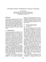
In this section, we introduce the general framework of the Bayesian HARDI atlas
estimation, as illustrated in Figure 4.2. Given n observed ODF datasets J (i) for i =
1, . . . , n, we assume that each of them can be estimated through an unknown atlas Iatlas
and a diffeomorphic transformation φ(i) such that
J (i) ≈ I (i) = φ(i) · Iatlas .

61

(4.1)


4. BAYESIAN ESTIMATION OF WHITE MATTER ATLAS FROM HIGH
ANGULAR RESOLUTION DIFFUSION IMAGING

The total variation of J (i) relative to I (i) is then denoted by σ 2 . The goal here
is to estimate the unknown atlas Iatlas and the variation σ 2 . To solve for the unknown atlas Iatlas , we first introduce an ancillary “hyperatlas” I0 , and assume that
our atlas is generated from it via a diffeomorphic transformation of φ such that
Iatlas = φ · I0 . We use the Bayesian strategy to estimate φ and σ 2 from the set of
observations J (i) , i = 1, . . . , n by computing the maximum a posteriori (MAP) of
fσ (φ|J (1) , J (2) , . . . , J (n) , I0 ). This can be achieved using the Expectation-Maximization
algorithm by first computing the log-likelihood of the complete data (φ, φ(i) , J (i) , i =
1, 2, . . . , n) when φ(1) , · · · , φ(n) are introduced as hidden variables. We denote this likelihood as fσ (φ, φ(1) , . . . , φ(n) , J (1) , . . . J (n) |I0 ). We consider that the paired information
of individual observations, (J (i) , φ(i) ) for i = 1, . . . , n, as independent and identically
distributed. As a result, this log-likelihood can be written as
log fσ (φ, φ(1) , . . . , φ(n) , J (1) , . . . J (n) |I0 )
n

= log f (φ|I0 ) +

(4.2)

log f (φ(i) |φ, I0 ) + log fσ (J (i) |φ(i) , φ, I0 ) ,

i=1

where f (φ|I0 ) is the shape prior (probability distribution) of the atlas given the hyperatlas, I0 . f (φ(i) |φ, I0 ) is the distribution of random diffeomorphisms given the estimated
atlas (φ · I0 ). fσ (J (i) |φ(i) , φ, I0 ) is the conditional likelihood of the ODF data given its
corresponding hidden variable φ(i) and the estimated atlas (φ · I0 ). In the remainder
of this section, we first adopt f (φ|I0 ) and f (φ(i) |φ, I0 ) introduced in [61, 65] and then
describe how to calculate fσ (J (i) |φ(i) , φ, I0 ) in §4.3 based on a Riemannian structure of
the ODFs.

62


4.2 The Shape Prior of the Atlas and the Distribution of Random
Diffeomorphisms

Figure 4.2: Illustration of the general framework of the Bayesian HARDI atlas estimation.

4.2

The Shape Prior of the Atlas and the Distribution
of Random Diffeomorphisms

Adopting previous work [61, 65] , we discuss the construction of the shape prior
(probability distribution) of the atlas, f (φ|I0 ), under the framework of large deformation
diffeomorphic metric mapping (LDDMM, reviewed in §2.2). By the conservation law
of momentum in §2.2.2, we can compute the prior f (φ|I0 ) via m0 , i.e.,

f (φ|I0 ) = f (m0 |I0 ) ,

63

(4.3)


4. BAYESIAN ESTIMATION OF WHITE MATTER ATLAS FROM HIGH
ANGULAR RESOLUTION DIFFUSION IMAGING

where m0 is initial momentum defined in the coordinates of I0 such that it uniquely
determines diffeomorphic geodesic flows from I0 to the estimated atlas. When I0
remains fixed, the space of the initial momentum m0 provides a linear representation of
the nonlinear diffeomorphic shape space, Iatlas , in which linear statistical analysis can
be applied. Hence, assuming m0 is random, we immediately obtain a stochastic model
for diffeomorphic transformations of I0 . More precisely, we follow the work in [61, 65]
and make the following assumption.
Assumption 1. (Gaussian Assumption on m0 )

m0 is assumed to be a centered

Gaussian random field (GRF) model where the distribution of m0 is characterized by
its covariance bilinear form, defined by
Γm0 (v, w) = E m0 (v)m0 (w) ,

where v, w are vector fields in the Hilbert space of V with reproducing kernel kV .
−1
1
We associate Γm0 with kV . The “prior” of m0 in this case is then Z exp − 1 m0 , kV m0
2

2

where Z is the normalizing Gaussian constant. This leads to formally define the “logprior” of m0 to be
log f (m0 |I0 ) ≈ −

1
m0 , kV m0
2

2

,

(4.4)

where we ignore the normalizing constant term log Z.
We now consider the construction of the distribution of random diffeomorphisms,
f (φ(i) |φ, I0 ). Similar to the construction of the atlas shape prior, we define f (φ(i) |φ, I0 )
(i)

via the corresponding initial momentum m0 defined in the coordinates of φ · I0 . We

64

,


4.3 The Conditional Likelihood of the ODF Data
(i)

also assume that m0 is random, and therefore, we again obtain a stochastic model for
diffeomorphic transformations of Iatlas ∼ φ · I0 . We make the following assumption.
=
(i)

Assumption 2. (Gaussian Assumption on m0 )

(i)

m0 is assumed to be a centered

π
π
GRF model with its covariance as kV , where kV is the reproducing kernel of the smooth

vector field in a Hilbert space V .
Hence, we can define the log distribution of random diffeomorphisms as
log f (φ(i) |φ, I0 ) ≈ −

1 (i) π (i)
m ,k m
2 0 V 0

2

.

(4.5)

where as before, we ignore the normalizing constant term log Z.

4.3

The Conditional Likelihood of the ODF Data

In this section, we will derive the construction of the conditional likelihood of the
ODF data fσ (J (i) |φ(i) , φ, I0 ). From the field of information geometry [82], the space
of ODFs, p(s), forms a Riemannian manifold with the Fisher-Rao metric (reviewed
in §2.1). In our study, we choose the square-root representation of the ODFs as the
parameterization of the ODF Riemannian manifold, which was used recently in ODF
processing and registration [1, 80, 102]. We refer the interested reader to §2.1 for a
more detailed description of the Riemmanian manifold Ψ lies on. We denote J (i) as
ψ (i) (s, x), s ∈ S2 , x ∈ Ω in the remainder of the section. Similarly, we have the atlas
Iatlas = ψatlas (s, x), where ψatlas (s, x) not only represents the mean anatomical shape
characterized through the diffeomorphism but the mean ODF at each spatial location
√
described using ODF.
(i)

Given φ1 and ψatlas (s, x) at a specific spatial location x, we assume that ψ (i) (s, x)

65


4. BAYESIAN ESTIMATION OF WHITE MATTER ATLAS FROM HIGH
ANGULAR RESOLUTION DIFFUSION IMAGING

is generated through an exponential map, i.e., ,
ψ (i) (s, x) = expφ(i) ·ψatlas (s,x) ξ(x) ,

(4.6)

1

where the tangent vectors ξ(x) ∈ Tφ(i) ·ψatlas (s,x) Ψ lie in a linear space. Therefore, in
1

order to model conditional likelihood of the ODF fσ (J (i) |φ(i) , φ, I0 ), we make the
following assumption.

ξ(x) ∈ Tφ(i) ·ψatlas (s,x) Ψ is assumed to

Assumption 3. (Gaussian Assumption on ξ)

1

(i)

be a centered Gaussian Random Field on the tangent space of Ψ at φ1 · ψatlas (s, x). In
addition, we assume that this Gaussian random field has the covariance as σ 2 ΓId .

This assumption is based on previous works on Bayesian atlas estimation using images and shapes [61, 65]. The main difference here is that we assume that ξ(x) ∈
Tφ(i) ·ψatlas (s,x) Ψ is assumed to be a centered Gaussian Random Field on the tangent
1

space. We choose ΓId as the identity operator to be consistent with the inner product of
√
(i)
ODF defined in Eq. (2.2). The group action of the diffeomorphism, φ1 · ψatlas (s, x),

involves both the spatial transformation and reorientation of the ODF. Based on the
equation (3.10) in Chapter 3, we define this group action as
⎛

(i) −1

(i)

φ1 · ψatlas (s, x) =

det D(φ(i) )−1 φ1
1

3
(i) −1
s
D(φ(i) )−1 φ1
1

ψatlas ⎝

(i) −1

s

(i) −1

s

(D(φ(i) )−1 φ1

1

(D(φ(i) )−1 φ1
1

⎞
(i)

, (φ1 )−1 (x)⎠ . (4.7)

This leads to formally define the “log-likelihood” of ξ(x) as
−

1
ξ, ξ
2σ 2

2

=−

1
logφ(i) ·ψatlas (s,x) ψ (i) (s, x)
1
2σ 2

2
(i)

φ1 ·ψatlas (s,x)

.

From the Gaussian assumption, we can thus write the conditional “log-likelihood” of

66


4.4 Expectation-Maximization Algorithm
(i)

J (i) given Iatlas and φ1 as
(i)

log fσ (J (i) |φ1 , φ1 , I0 )
≈

x∈Ω

−

(4.8)

1
logφ(i) ·ψatlas (s,x) ψ (i) (s, x)
1
2σ 2

2

−

(i)

φ1 ·ψatlas (s,x)

log σ 2
dx ,
2

where as before, we ignore the normalizing Gaussian term, and I0 is denoted as ψ0 (s, x)
such that ψatlas (s, x) = φ1 · ψ0 (s, x).

4.4

Expectation-Maximization Algorithm

We have shown how to compute the log-likelihood shown in Eq. (4.2) in §4.1 and §4.3.
In this section, we will show how we employ the Expectation-Maximization algorithm
to estimate the atlas, Iatlas = ψatlas (s, x), for s ∈ S2 , x ∈ Ω, and σ 2 . From the above
discussion, we first rewrite the log-likelihood function of the complete data in Eq. (4.2)
as
log fσ (φ, φ(1) , . . . , φ(n) , J (1) , . . . J (n) |I0 )
(1)

(4.9)

(n)

≈ log fσ (m0 , m0 , . . . , m0 , ψ (1) , . . . ψ (n) |ψ0 )

1
m0 , kV m0 2
2
n
1 (i) π (i)
m , k V m0
−
2 0
i=1

≈−

2

+
x∈Ω

1
logφ(i) ·ψatlas (s,x) ψ(s, x)
1
2σ 2

2
(i)

φ1 ·ψatlas (s,x)

+

log σ 2

dx
2

,

where ψatlas (s, x) = φ1 · ψ0 (s, x) and can be computed based on Eq. (4.7).
The E-Step. The E-step computes the expectation of the complete data log-likelihood
old

given the previous atlas mold and variance σ 2 . We denote this expectation as
0
old

Q(m0 , σ 2 |mold , σ 2 ) given in the equation below,
0
Q m0 , σ 2 |mold , σ 2
0

old

(4.10)

67


4. BAYESIAN ESTIMATION OF WHITE MATTER ATLAS FROM HIGH
ANGULAR RESOLUTION DIFFUSION IMAGING

(1)

(n)

old

log fσ (m0 , m0 , . . . , m0 , ψ (1) , . . . ψ (n) |ψ0 ) mold , σ 2 , ψ (1) , · · · , ψ (n) , ψ0
0

=E

1
m0 , kV m0 2
2
n
1 (i) π (i)
m , kV m0
−
E
2 0
i=1

≈−

+

2

x∈Ω

1
logφ(i) ·ψatlas (s,x) ψ (i) (s, x)

1
2σ 2

2
(i)

φ1 ·ψatlas (s,x)

+

log σ 2
dx .
2

The M-Step. The M-step generates the new atlas by maximizing the Q-function with
respect to m0 and σ 2 . The update equation is given as
mnew , σ 2
0

new

(4.11)

= arg max Q m0 , σ 2 |mold , σ 2
0

old

m0 ,σ 2

n

= arg min
m0 ,σ 2

m0 , k V m0

2

+

E

x∈Ω

i=1

1
logφ(i) ·ψatlas (s,x) ψ (i) (s, x)
1
σ2

2
(i)

φ1 ·ψatlas (s,x)

(i)

(i)

π
where we use the fact that the conditional expectation of m0 , kV m0

2

+ log σ 2 dx

is constant.

We solve σ 2 and m0 by separating the procedure for updating σ 2 using the current value
of m0 , and then optimizing m0 using the updated value of σ 2 .
Thus, we can show that it yields the following update equations (the proof is shown
later in §4.4.1),
σ

2 new

1
=
n

n
x∈Ω

i=1

mnew = arg min
0

(i)

φ1 ·ψatlas (s,x)

1

m0 , kV m0

m0

2

logφ(i) ·ψatlas (s,x) ψ (i) (s, x)
2

+

1
σ 2new

x∈Ω

dx ,

(4.12)

α(x) logψ0 (s,x) φ1 · ψ0 (s, x)

2
ψ 0 (s,x)

dx

,
(4.13)

n

where α(x) =

(i)

|Dφ1 (x)| is a weighted image volume to control the contribution of
i=1

(i)

the HARDI matching errors to the total cost at each voxel level. |Dφ1 | is the Jacobian
(i)

determinant of φ1 . The mean ODF ψ 0 (s, x) is defined as the solution to the following

68

,


4.4 Expectation-Maximization Algorithm

minimization problem

1
ψ 0 (s, x) = arg min
2
ψ∈Ψ

n
i=1

(i)

|Dφ1 (x)|

n
j=1

(i)

(j)
|Dφ1 (x)|

logψ(s,x) (φ1 )−1 · ψ (i) (s, x)

ψ(s,x)

.

(4.14)
To compute ψ 0 (s, x), the weighed Karcher mean algorithm given in [1] is used. In
addition, from [1], we also know that ψ 0 (s, x) is the unique solution to
1

n
j=1

n

(j)
|Dφ1 (x)| i=1

(i)

(i)

|Dφ1 (x)| logψ0 (s,x) (φ1 )−1 · ψ (i) (s, x) = 0.

(4.15)

The variational problem listed in Eq. (4.13) is referred as “modified LDDMM-ODF
mapping”, where the weight α is introduced. We now present the steps involved in each
iteration in Algorithm 1.

Algorithm 1 (The EM Algorithm for the HARDI Atlas Generation)
We initialize m0 = 0. Thus, the hyperatlas ψ0 is considered as the initial atlas.
1. Apply the LDDMM-ODF mapping algorithm in Chapter 3 to register the current
(i)
(i)
atlas to each individual HARDI dataset, which yields m0 and φt .
2. Compute ψ 0 according to Eq. (4.14) using the weighted Karcher mean algorithm
given in [1].
3. Update σ 2 according to Eq. (4.12).
4. Estimate ψatlas = φ1 · ψ0 , where φt is found by applying the modified LDDMMODF mapping algorithm as given in Eq. (4.13).

The above computation is repeated until the atlas converges.

69


4. BAYESIAN ESTIMATION OF WHITE MATTER ATLAS FROM HIGH
ANGULAR RESOLUTION DIFFUSION IMAGING

4.4.1

Derivation of Update Equations of σ 2 and m0 in EM

We now derive Eqs. (4.12) and (4.13) from Q-function in Eq. (4.10) for updating
values of σ 2 and m0 . The reader can skip this subsection without loss of continuity by
assuming that Eqs. (4.12) and (4.13) hold ture. It is straightforward to obtain σ 2 by
taking the derivative of Q m0 , σ 2 |mold , σ 2
0
(i)

For updating m0 , let y = φ1

x∈Ω

−1

old

with respect to σ 2 and setting it to zero.

(x). By the change of variables strategy, we have

logφ(i) ·ψatlas (s,x) ψ (i) (s, x)
1

2
(i)

φ1 ·ψatlas (s,x)

(i)

=
y∈Ω

logψatlas (s,y) (φ1 )−1 · ψ (i) (s, y)

dx

2

(4.16)
(i)

ψatlas (s,y)

|Dφ1 (y)|dy .

Therefore, we can then rewrite

n

E
i=1
n

=

E
i=1

x∈Ω

y∈Ω

y∈Ω

1
2σ 2

y∈Ω

1
2σ 2

y∈Ω

1
2σ 2

=

(a)

≈

=

1
logφ(i) ·ψatlas (s,x) ψ (i) (s, x)
1
2σ 2

2
(i)

φ1 ·ψatlas (s,x)

1
(i)
logψatlas (s,y) (φ1 )−1 · ψ (i) (s, y)
2σ 2

n

(i)

dx

2

(i)

ψatlas (s,y)
2

|Dφ1 (y)|dy
(i)

E

logψatlas (s,y) (φ1 )−1 · ψ (i) (s, y)

E

logψ0 (s,y) (φ1 )−1 · ψ (i) (s, y) − logψ0 (s,y) ψatlas (s, y)

i=1
n
i=1
n

E
i=1

ψatlas (s,y)

|Dφ1 (y)| dy

(i)

(i)

logψ0 (s,y) (φ1 )−1 · ψ (i) (s, y)

2
ψ 0 (s,y)

ψ 0 (s,y)

(i)

|Dφ1 (y)| dy
2

+ logψ0 (s,y) ψatlas (s, y)

(i)

− 2 logψ0 (s,y) (φ1 )−1 · ψ (i) (s, y) , logψ0 (s,y) ψatlas (s, y)

2

ψ 0 (s,y)

(i)

ψ 0 (s,y)

|Dφ1 (y)| dy

(i)

where (a) is the first order approximation of logψatlas (s,y) (φ1 )−1 ·ψ (i) (s, y)

2
ψatlas (s,y)

.

As the direct consequence of the Karcher mean definition of ψ 0 (s, y) in Eq. (4.14),
and more precisely Eq. (4.15),

n
i=1

(i)

(i)

|Dφ1 (x)| logψ0 (s,x) (φ1 )−1 · ψ (i) (s, x) = 0,

70


4.5 Results

the above cross item is equal to zero. Therefore, we get

y∈Ω

1

2σ 2

n

(i)

logψ0 (s,y) (φ1 )−1 · ψ (i) (s, y)

E
i=1

+ logψ0 (s,y) ψatlas (s, y)

2
ψ 0 (s,y)

2
ψ 0 (s,y)
(i)

|Dφ1 (y)| dy.

Since the first item in the above equation is independent of m0 , we have
mnew = arg min m0 , kV m0
0
m0

where α(y) =

4.5

n
i=1

2

+

1
σ 2new

y∈Ω

α(y) logψ0 (s,y) φ1 · ψ0 (s, y)

2
ψ 0 (s,y)

dy ,

(i)

|Dφ1 (y)|. By changing y by x, we obtain Eq. (4.12).

Results

In this section, we demonstrate the performance of the probabilistic HARDI atlas
generation algorithm proposed on real human data. In §4.5.1, we show the HARDI atlas
based on 94 healthy adults. §4.5.2 empirically examines the convergence of the HARDI
atlas estimation procedure and studies the effects of the choice of the hyperatlas, which

is used as the initial atlas in Algorithm 1, on the final estimated atlas. §4.5.3 shows the
estimated atlases across different age groups. Finally, §4.5.4 compares our proposed
algorithm to an existing algoritim in [68].
Subjects and Image Acquisition: 94 participants were recruited through advertisements posted at the National University of Singapore (NUS). 38 males and 56 females
ranged from 22 to 71 years old (mean ± standard deviation (SD): 42.5 ± 13.9 years)
participated in the study. A health screening questionnaire along with informed consent
approved by the NUS Institutional Review Board was acquired from each participant.

71


4. BAYESIAN ESTIMATION OF WHITE MATTER ATLAS FROM HIGH
ANGULAR RESOLUTION DIFFUSION IMAGING

Any participant with a history of psychological, neurological disorder or surgical implantation was excluded from the study. A Mini Mental Status Examination (MMSE)
was administered to each participant to rule out possible cognitive impairments. All
participants had the MMSE score greater than 26.
Every participant underwent magnetic resonance imaging scans that were performed
on a 3T Siemens Magnetom Trio Tim scanner using a 32-channel head coil at Clinical
Imaging Research Center at the NUS. The image protocols were: (i) isotropic high
angular resolution diffusion imaging (single-shot echo-planar sequence; 48 slices of
3mm thickness; with no inter-slice gaps; matrix: 96 × 96; field of view: 256 × 256mm;
repetition time: 6800 ms; echo time: 85 ms; flip angle: 90◦ ; 91 diffusion weighted
images (DWIs) with b = 1150 s/mm2 , 11 baseline images without diffusion weighting);
(ii) isotropic T2-weighted imaging protocol (spin echo sequence; 48 slices with 3 mm
slice thickness; no inter-slice gaps; matrix: 96 × 96; field of view: 256 × 256 mm;
repetition time: 2600 ms; echo time: 99 ms; flip angle: 150◦ ).

HARDI Preprocessing: DWIs of each subject were first corrected for motion and
eddy current distortions using affine transformation to the image without diffusion

weighting. Within-subject, we followed the procedure detailed in [103] to correct
geometric distortion of the DWIs due to b0-susceptibility differences over the brain.
Briefly reviewing, the T2-weighted image was considered as the anatomical reference.
The deformation that carried the baseline image without diffusion weighting to the T2weighted image characterized the geometric distortion of the DWI. For this, intra-subject
registration was first performed using FLIRT [104] to remove linear transformation
(rotation and translation) between the diffusion weighted images and T2-weighted
image. Then, LDDMM [93] sought the optimal nonlinear transformation that deformed

72


4.5 Results

the baseline image without the diffusion weighting to the T2-weighted image. This
diffeomorphic transformation was then applied to every diffusion weighted image in
order to correct the nonlinear geometric distortion. Existing literature [92, 99] have
proposed different ways of reorienting the diffusion gradients. In this work, the diffusion
gradients are reoriented using the method proposed in [92]. Briefly speaking, if φ is
the diffeomorphism, then the local affine transformation Ax at spatial coordinates x is
defined as the Jacobian matrix of φ evaluated at x. If gi is the ith diffusion gradient, then
the reoriented diffusion gradient after the affine transformation Ax is simply

A − gi
x
A − gi
x

.

Finally, we estimated the ODFs using the approach considering the solid angle constraint

based on DWI images proposed in [48].

4.5.1

HARDI Atlas Generation

To initialize the HARDI atlas generation process, we chose the HARDI dataset of
one participant (male, 43 years old) as hyperatlas and assumed m0 = 0 such that the
hyperatlas was used as the initial atlas. We select this participant because his age is
around the average age for the HARDI dataset. We then followed Algorithm 1 and ten
π
iterations were repeated. Notice that kV associated with the covariance of m0 and kV
(i)

associated with the covariance of m0 were assumed to be known and predetermined.
Since we were dealing with vector fields in R3 , the kernel of V is a matrix kernel
operator in order to get a proper definition. Making an abuse of notation, we defined kV
π
π
and kV respectively as kV Id3×3 and kV Id3×3 , where Id3×3 is a 3 × 3 identity matrix
π
π
and kV and kV are scalars. In particular, we assumed that kV and kV are Gaussian with

kernel sizes of σV and σV π . Since σV determines the smoothness level of the mapping
from the hyperatlas to the blur ψ 0 (s, x) whereas σV π determines that from the sharp

73

4. BAYESIAN ESTIMATION OF WHITE MATTER ATLAS FROM HIGH
ANGULAR RESOLUTION DIFFUSION IMAGING

atlas to individual HARDI datasets, σV should be greater than σV π . We experimentally
determined σV π = 5 and σV = 8.
Figure 4.3 shows the evolution of ψ 0 (s, x) over the iterations of the EM algorithm.
As seen in Figure 4.3, the white matter anatomy of ψ 0 (s, x) was blur at the initial
estimate and became sharper as more iterations were run. Figure 4.4 illustrates the atlas
estimated from the 94 adults’ HARDI datasets after ten iterations. Panels (a-c) shows
the coronal view of the atlas, while panels (d-f) and (g-i) respectively illustrate the axial
and sagittal views of the atlas. The branching and crossing bundles in the estimated
atlases over the entire population group illustrate that the atlas preserves the anatomical
details of the white matter.

Figure 4.3: The evolution of ψ 0 (s, x) over the optimization of the atlas estimation. Panels
from left to right show ψ 0 (s, x) before the optimization, at the first, fifth, and tenth
√
iterations, respectively. The intensity indicates the ODF metric of each voxel with respect
to the spherical ODF. The larger the value, the more anisotropic the ODF is.

4.5.2

Convergence and Effects of Hyperatlas Choice of the HARDI
Atlas Estimation

In this section, we empirically demonstrate the convergence of the average diffeomorphic metric of individual subjects when referenced to the estimated atlas. This is
measured using the square root of the inner product of the initial momentum. Figure

74

4.5 Results

4.5 shows the evolution of the average diffeomorphic metric of individual subjects
referenced to the estimated atlas as well as the standard deviation across the subjects.
From Figure 4.5, we see that the average diffeomorphic metric changed less than 5%
after two iterations. In addition, Table 4.1 shows that the total variance of the observed
HARDI datasets, ψ (i) , i = 1, 2, . . . , n, relative to the estimated atlas became stable
after seven iterations as well. The computational time for each LDDMM-ODF mapping
was about 30 minutes.
√
Table 4.1: Convergence of the atlas quantified through the ODF metric square between
the atlases estimated at the current and previous iteration and σ 2 in each iteration of the
atlas estimation.
(k)

(k−1)

Iteration dist(ψatlas , ψatlas )2
1
303.42
2
42.39
3
4.80
4
0.96
5
1.06
6

0.18
7
0.01
8
0.01
9
0.01
10
0.01

(k)

σ 2 (×10−3 )
3.05
1.80
1.40
1.38
1.39
1.39
1.39
1.39
1.39
1.39

Next, we study the effects of the hyperatlas choice on the estimated atlas. In the
Bayesian modeling for the HARDI atlas generation presented here, the hyperatlas ψ0 is
assumed to be known and fixed. In addition, the hyperatlas is used as the initialization
for the atlas in the EM algorithm. Therefore, the anatomy of the estimated atlas can be
dependent on the choice of the hyperatlas. In this section, we demonstrate the influence
due to the hyperatlas.

We repeated the atlas estimation procedure when two different HARDI datasets,

75


4. BAYESIAN ESTIMATION OF WHITE MATTER ATLAS FROM HIGH
ANGULAR RESOLUTION DIFFUSION IMAGING

shown in Figure 4.6 (a, c), are respectively used as the hyperatlas. In this experiment,
instead of using the entire dataset of 94 adults, only ten HARDI datasets were chosen
from our sample pool as the observables, ψ (i) , i = 1, 2, . . . , 10. Figure 4.6 (b, d) show
the estimated HARDI atlases obtained from the hyperatlases shown in Figure 4.6 (a,
c), respectively. As seen in Figure 4.6 (e), differences between the two hyperatlases
√
are large in terms of the ODF metric square even in major white matter bundles
(e.g., corpus callosum, external capsule). Nevertheless, Figure 4.6 (f), which shows the
√
ODF metric square between the estimated two atlases, illustrates that they are similar.
A two-sample Kolmogorov-Smirnov test revealed that the cumulative distribution of the
√
ODF metric square as shown in Figure 4.7 between the two estimated atlases (Figure
4.6 (b, d)) is significantly greater than that between the two hyperatlases (Figure 4.6 (a,
√
c)) (p < 0.001), which indicates that more voxels with small ODF between the two
estimated atlases when compared to those between the two hyperatlases. This result
suggests that the choice of the hyperatlas has minimal effects on the resulting estimated
atlas.

76

4.5 Results

Figure 4.4: Illustration of the branching and crossing bundles in the estimated atlases over
the entire population group. Panels (a,d,g) show the ODF field in the coronal, axial, and
sagittal views. In each row, the second and third panels show two zoom-in regions for
branching and crossing bundles corresponding to the anatomy on the first panel.

77


4. BAYESIAN ESTIMATION OF WHITE MATTER ATLAS FROM HIGH
ANGULAR RESOLUTION DIFFUSION IMAGING

Metric distance to estimated atlas

Deviation of individual data to estimated atlas
Mean (SD error bars)

3
2.5
2
1.5
1
0

2

4

6
Iteration

8

10

Figure 4.5: The evolution of the average diffeomorphic metric between individual subjects
and the estimated atlas, with the standard deviation shown by the error bars.

78


4.5 Results

Figure 4.6: Influences of the hyperatlas on the estimated atlas. Two HARDI datasets
(panels (a, c)) were respectively used as the hyperatlas in the Bayesian atlas estimation,
√
which generated the atlases shown in panels (b, d). Panel (e) shows the ODF metric
square between the two hyperatlases on (a, c), while panel (f) shows that between the atlases
on (b, d).

79


4. BAYESIAN ESTIMATION OF WHITE MATTER ATLAS FROM HIGH
ANGULAR RESOLUTION DIFFUSION IMAGING

1

Percentage

0.98
0.96
0.94
hyperatlas
estimated atlas

0.92
0.9
0.0

0.1

0.2

0.3

ODF Metric Difference

√
Figure 4.7: The cumulative distributions of the ODF metric square between the two
hyperatlases (Figure 4.6 (a, c)) and between the two estimated atlases (Figure 4.6 (b, d))
are respectively shown in the dashed and solid lines. For each voxel, the red (metric=0.1)
indicts the difference between the template and the deformed subjects is large, while the
blue (metric=0) indicts the two corresponding ODFs are equal.

80

4.5 Results

4.5.3

Aging HARDI atlases

In this section, we performed our HARDI atlas generation process on two different age
groups, young and old adults, and demonstrated that the estimated atlas of each specific
age group exhibits characteristics of the group that are in line with what is reported in
current literature.
We selected a subset of the dataset and divided them into two groups. In the young
adults group, there were 21 subjects (8 males and 13 females) ranging from 22 to
39 years old (mean ± standard deviation (SD): 27.6 ± 4.28 years); In the old adults
group, there were also 21 subjects (9 males and 12 females) ranging from 55 to 71
years old (mean ± standard deviation (SD): 61.90 ± 3.81 years). Next, we choose one
subject (male, 24 years old) as the hyperatlas for the young adults group and another
subject (male, 71 years old) for the old adults group, and performed the proposed atlas
generation algorithm shown in Algorithm 1 for each of the two groups.
In Figure 4.8, three regions of interest are selected for comparison between the
atlases for young and old adults groups. For the regions of the corpus callosum and
ventricles in Panel 4.8(c) and 4.8(g), the most obvious aging effect observed is the
bending of the corpus callosum due to the enlargement of ventricles, together with
the thinning of the corpus callosum, which is consistent with previous findings in
[69, 70, 71]. For the region of the branching fibers, Panel 4.8(b) and 4.8(f) show that
there are more branches in the atlas of young adults group than those in the one of old
adults group. The similar effect is also observed in the region of the crossing fibers
in Panel 4.8(d) and 4.8(h). A detailed comparison of the ODF shape explains that
the anisotropy for the ODFs declines with advancing age due to the fact that axons’
distribution becomes more uniform as age increases. This ODF shape differences could

81


4. BAYESIAN ESTIMATION OF WHITE MATTER ATLAS FROM HIGH
ANGULAR RESOLUTION DIFFUSION IMAGING

be due to the breakdown of the myelin sheath with aging and increases in extracellular
fluid and transverse diffusivity as suggested in [105].
(a) Young Adults

(e) Old Adults

(b) Young: Branching (c) Young: Corpus Cal- (d) Young:
Fibers
losum
Fibers

(f) Old:
Fibers

Crossing

Branching (g) Old: Corpus Callo(h) Old: Crossing Fibers
sum

Figure 4.8: Comparison of HARDI atlases respectively generated from young and old
adults. In each row, the last three columns show three zoom-in regions for branching and
crossing bundles corresponding to the anatomy given on the first panel.

4.5.4

Comparison with existing method

In this section, we compared our proposed method with the one proposed in [68]. In
the rest of this section, we referred the atlas generated from our proposed method as
Bayesian atlas, and the one from [68] as averaged atlas. While the code used in [68]
is not publicly available, we manage to adapt it into the same LDDMM framework as
our proposed method. To implement the ODF-based registration algorithm in [68], we
minimized the mean square error (MSE) of the spherical harmonic coefficients (SHC) of
ODFs between the warped atlas and subjects, and then applied the finite strain scheme,

82


4.6 Summary

which only keeps the rotation part of the local Jacobian field, to reorientate the ODFs.
To generate an average atlas for the dataset, we first selected the same subject as the
hyperatlas, and warped each subject into the hyperatlas space using by the registration
method we describe above. Finally, we generated the average atlas by averaging the
SHC across all the warped subjects. For a fair comparison, we kept all other conditions
the same for the generation of both Bayesian and averaged atlases, and conducted the
experiments by selecting the same hyperatlas for the entire dataset.
As shown in Figure 4.9, the ODFs in the Bayesian atlas is generally much sharper
than those in the averaged atlas. Moreover, as demonstrated in Panel 4.9(b) and 4.9(f),
some small branches can only be revealed in the Bayesian atlas, while they cannot be
found in the averaged atlas due to the averaging process. Furthermore, in the region
of crossing fibers shown in Panel 4.9(c) and 4.9(g), the Bayesian atlas preserved more
details than the averaged atlas. However, there was not much difference in the main
fiber tract as illustrated in Panel 4.9(d) and 4.9(h).

4.6

Summary

In this chapter, we present a Bayesian model to estimate the white matter atlas from
observed HARDI datasets under the LDDMM framework. To the best of our knowledge,
this is the first probabilistic approach for the HARDI atlas generation. In this work, we
construct the ODF likelihood function based on its Riemannian structure. In particular,
we employ the square root parameterization of the ODF Riemannian manifold such that
the logarithmic and exponential maps are in closed forms. This facilitates the construction of the ODF likelihood through the tangent vector of the ODF, i.e., logarithmic map,
lying in a linear space where linear statistical models can be applied. We further derive

83