Registration, atlas generation, and statistical analysis of high angular resolution diffusion imaging based on riemannian structure of orientation distribution functions 5
Bạn đang xem bản rút gọn của tài liệu. Xem và tải ngay bản đầy đủ của tài liệu tại đây (808.27 KB, 26 trang )
5
Geodesic Regression of Orientation
Distribution Functions with its
Application to Aging Study
After the HARDI dataset across a population has been warped into the common atlas,
the non-linear nature of HARDI data presents a challenge to HARDI-based statistical
analysis (see Figure 5.1). Regression analysis is a fundamental statistical tool to
determine how a measured variable is related to one or more independent variables.
The most widely used regression model is linear regression, because of its simplicity,
ease of interpretation, and ability to model many phenomena. However, if the response
variable takes values in a nonlinear manifold, a linear model is not applicable. Such
manifold-valued measurements arise in many applications, including those that involve
directional data, transformations, tensors, and shapes. Several works have studied the
regression problem on manifolds e.g., [
69
,
70
]. In this chapter, we adapt the framework
of geodesic regression, proposed in [
70
], to the HARDI data and apply it to the aging
85
5. GEODESIC REGRESSION OF ORIENTATION DISTRIBUTION
FUNCTIONS WITH ITS APPLICATION TO AGING STUDY
study. First we derive the algorithm for the geodesic regression on Riemannian manifold
of ODFs and conduct the simulation experiment to evaluate its performance. Finally,
we examine the effects of aging via geodesic regression of ODFs in a large group of
healthy men and women, spanning the adult age range.
HARDI
data
ODF
images
ODF
images
in common
space
ODF
atlas
ODF
Reconstruction
Registration
Atlas
Generation
Biomarkers/
Inference
Statistical
Analysis
serve as
common
space in
registration
Subjects
Data
Acquisition
Figure 5.1: The role of Chapter 5 in the ODF-based analysis framework.
5.1 Geodesic Regression on the ODF manifold
In statistics, the simple linear regression is an approach to modeling the relationship
between a scalar dependent variable
Y
and a non-random scalar variable denoted as
X
.
86
5.1 Geodesic Regression on the ODF manifold
A linear regression model of this relationship can be given as
Y = β
0
+ β
1
X + , (5.1)
where
β
0
is an unknown intercept parameter,
β
1
is an unknown slope parameter, and
is an unknown random variable representing the error drawn from distributions with
zero mean and finite variance. Given
n
observations, i.e.,
(x
i
,y
i
),
for
i =1, 2, ···,n
,
the least square estimates,
ˆ
β
0
and
ˆ
β
1
, for the intercept and slope can be computed by
minimizing the square errors
(
ˆ
β
0
,
ˆ
β
1
) = arg min
(β
0
,β
1
)
n
i=1
y
i
− β
0
− β
1
x
i
2
. (5.2)
This minimization problem can be analytically solved. The observations,
y
i
can be
approximated as
ˆy
i
=
ˆ
β
0
+
ˆ
β
1
x
i
,i=1, 2, ···,n.
We will now extend the above simple linear regression to the one modeling the
relationship of the ODF and one non-random scalar variable,
X
, by adopting the general
framework of geodesic regression in [70, 81].
We now formulate the geodesic regression that models the relationship of a
Ψ
-valued
random variable
Ψ
and a non-random variable
X ∈ R
. Such a geodesic relationship
cannot be simply written as the summation of the intercept
β
0
and the scalar variable
X
weighted by
β
1
, where
β
0
and
β
1
are scalar measures as shown in Eq.
(5.1)
. Rather,
in this case (see Figure 5.2), it needs to be adopted to the manifold setting in which
the exponential map in Eq.
(2.4)
will be used to replace the addition in the Euclidean
space. Hence, we introduce the parameters
ψ
and
ξ
, where
ψ
is an element on
Ψ
and
87
5. GEODESIC REGRESSION OF ORIENTATION DISTRIBUTION
FUNCTIONS WITH ITS APPLICATION TO AGING STUDY
ξ ∈ T
ψ
Ψ
is a tangent vector at
ψ
on
Ψ
. This pair of parameters
(ψ, ξ)
provides an
intercept
ψ
and a slope
ξ
, analogous to the
β
0
and
β
1
parameters in the simple linear
regression in Eq. (5.1). The geodesic regression model can thus be written as
Ψ=exp
exp(ψ,Xξ),
, (5.3)
where
is a random variable taking values in the tangent space at
exp(ψ,Xξ)
. Notice
that in a Euclidean space, the exponential map is simply addition, i.e.,
exp(ψ,Xξ)=
ψ+Xξ
. Thus, when the manifold is a Euclidean space, the geodesic model is equivalent
to the simple linear regression in Eq.
(5.1)
. Hence, the geodesic regression is the
generalization of the simple linear regression to the manifold setting.
Figure 5.2: Geodesic regression on manifold Ψ.
88
5.1 Geodesic Regression on the ODF manifold
5.1.1 Least-Squares Estimation and Algorithm
Given
n
observations,
(x
i
, ψ
i
) ∈ R × Ψ
,
i =1, 2, ···,n
, we estimate
(ψ, ξ)
via
solving a least-squares problem by computing the least-squares estimates
ˆ
ψ
and
ˆ
ξ
,
which minimizes
E(ψ, ξ)=
n
i=1
1
2
dist
ψ
i
, exp(ψ,x
i
ξ)
2
, (5.4)
where
dist(·, ·)
, given in Eq.
(2.3)
, is the geodesic metric distance between
ψ
i
and its
approximation
ˆ
ψ
i
=exp(ψ,x
i
ξ)
. Unlike the simple linear regression, this minimiza-
tion problem cannot be analytically solved. Therefore, we seek the estimates of
(ψ, ξ)
using a gradient descent algorithm. In order to do so, we have to derive the gradient of
E
with respect to
ψ
as well as with respect to
ξ
. We refer readers to
§
5.1.1.1 for the
detailed derivation of these two gradient terms.
Briefly, the gradient of
E
with respect to
ψ
(see Eq. 5.7), denoted as
∇
ψ
E
, can be
written as
∇
ψ
E = −
n
i=1
cos(x
i
ξ
ˆ
ψ
i
)log
ˆ
ψ
i
ψ
i
, (5.5)
Furthermore, the gradient of
E
with respect to
ξ
(see Eq. 5.8), denoted as
∇
ξ
E
, can
be written as
∇
ξ
E = −
n
i=1
x
i
log
ˆ
ψ
i
ψ
i
ˆ
ψ
i
ξ
ξ
ψ
+
sin(x
i
ξ
ψ
)
ξ
ψ
log
ˆ
ψ
i
ψ
i
⊥
, (5.6)
89
5. GEODESIC REGRESSION OF ORIENTATION DISTRIBUTION
FUNCTIONS WITH ITS APPLICATION TO AGING STUDY
where
log
ˆ
ψ
i
ψ
i
and
log
ˆ
ψ
i
ψ
i
⊥
are given as
log
ˆ
ψ
i
ψ
i
=
log
ˆ
ψ
i
ψ
i
,
ξ
i
ξ
i
ˆ
ψ
i
ˆ
ψ
i
ξ
i
ξ
i
ˆ
ψ
i
,
and
log
ˆ
ψ
i
ψ
i
⊥
=log
ˆ
ψ
i
ψ
i
−
log
ˆ
ψ
i
ψ
i
,
where ξ
i
is the parallel translation of ξ from ψ to
ˆ
ψ
i
, given as
ξ
i
= −sin
x
i
ξ
ψ
ξ
ψ
ψ +cos
x
i
ξ
ψ
ξ ,
and (·)
and (·)
⊥
denote components of (·) parallel and orthogonal to ξ
i
respectively.
We employ the gradient descent algorithm to find the minimizer to the least-squares
problem found in Eq.
(5.4)
. At the beginning of the optimization, we initialize
ξ =0
and
ψ
to be the Karcher mean of the observed ODF,
ψ
i
,i =1, 2, ···,n
, where the
Karcher mean is computed using the Karcher mean algorithm given in [
1
]. During each
iteration of the optimization, the estimates of
(ψ, ξ)
are respectively updated using
Eq.
(5.5)
and Eq.
(5.6)
. The above computation is repeated until the change of
E
is
sufficiently small.
5.1.1.1 Derivation of the Least-Squares Estimation
We now show how to compute the gradient of
E
in Eq.
(5.4)
with respect to the
intercept
ψ
and the slope
ξ
via the calculus of variation method. The reader can skip
this subsection without losing the flow of the exposition by assuming that the gradient
90
5.1 Geodesic Regression on the ODF manifold
of
E
in Eq.
(5.4)
holds ture. For the simplicity, we denote
ˆ
ψ
i
=exp(ψ,x
i
ξ)
in the
following derivation.
We first compute the gradient of
E
with respect to
ψ
, denoted as
∇
ψ
E
. Let
ψ
ε
=exp(ψ,εμ)
where
ε
is a scalar and
μ ∈ T
ψ
Ψ
is a tangent vector at
ψ
.Wenow
take the derivative of E at ε =0.Wehave
∂E
∂ε
ε=0
=
∂
∂ε
n
i=1
1
2
log
exp(ψ
ε
,x
i
ξ)
ψ
i
2
exp(ψ
ε
,x
i
ξ)
ε=0
=
n
i=1
log
ˆ
ψ
i
ψ
i
,
∂
∂ε
log
exp(ψ
ε
,x
i
ξ)
ψ
i
ε=0
ˆ
ψ
i
(a)
≈
n
i=1
− log
ˆ
ψ
i
ψ
i
,
∂
∂ε
exp(ψ
ε
,x
i
ξ)
ε=0
ˆ
ψ
i
=
n
i=1
− log
ˆ
ψ
i
ψ
i
,D
ψ
exp(ψ,x
i
ξ)μ
ˆ
ψ
i
=
n
i=1
−
D
ψ
exp(ψ,x
i
ξ)
†
log
ˆ
ψ
i
ψ
i
, μ
ψ
,
where
(a)
is obtained from the first order approximation of
log
exp(ψ
ε
,x
i
ξ)
ψ
i
based on
the Taylor expansion of the logarithm map.
D
ψ
exp(ψ,x
i
ξ)
is the operator that maps
μ
from the tangent space of
ψ
to that of
ˆ
ψ
i
. When we assume that
x
i
ξ
ψ
ε
= x
i
ξ
ψ
,
where
ε
is sufficiently small, this operator can be directly computed according to
the analytical form of the exponential map given in Eq.
(2.4)
and the first order
approximation of
exp(ψ,εμ)
based on the Taylor expansion of the exponential map.
This yields
D
ψ
exp(ψ,x
i
ξ) = cos(x
i
ξ
ψ
) .
It is self-adjoint. Its adjoint operator,
D
ψ
exp(ψ,x
i
ξ)
†
, maps
log
ˆ
ψ
i
ψ
i
from the
91
5. GEODESIC REGRESSION OF ORIENTATION DISTRIBUTION
FUNCTIONS WITH ITS APPLICATION TO AGING STUDY
tangent space of
ˆ
ψ
i
to that of ψ. Therefore,
∇
ψ
E = −
n
i=1
cos(x
i
ξ
ˆ
ψ
i
)log
ˆ
ψ
i
ψ
i
, (5.7)
Next, we compute the derivative of
E
with respect to
ξ
denoted as
∇
ξ
E
. Let
ξ
ε
= ξ + εμ
, where
ε
is a scalar and
μ ∈ T
ψ
Ψ
is a tangent vector at
ψ
. We now take
the derivative of E at ε =0.Wehave
∂E
∂ε
ε=0
=
∂
∂ε
n
i=1
1
2
log
exp(ψ,x
i
ξ
ε
)
ψ
i
2
exp(ψ,x
i
ξ
ε
)
ε=0
=
n
i=1
log
ˆ
ψ
i
ψ
i
,
∂
∂ε
log
exp(ψ,x
i
ξ
ε
)
ψ
i
ε=0
ˆ
ψ
i
(a)
≈
n
i=1
− log
ˆ
ψ
i
ψ
i
,
∂
∂ε
exp(ψ,x
i
ξ
ε
)
ε=0
ˆ
ψ
i
,
where
(a)
is obtained from the first order approximation of
log
exp(ψ,x
i
ξ
ε
)
ψ
i
based
on Taylor expansion of the logarithm map. According to the analytical form of the
exponential map given in Eq. (2.4), we have
∂
∂ε
exp(ψ,x
i
ξ
ε
)
ε=0
=
−sin(x
i
ξ
ψ
)ψ +cos(x
i
ξ
ψ
)
ξ
ξ
ψ
x
i
ξ
ξ
ψ
, μ
ψ
+
sin(x
i
ξ
ψ
)
ξ
ψ
μ −
ξ
ξ
ψ
, μ
ψ
ξ
ξ
ψ
For short, we denote
ξ
i
ξ
i
ˆ
ψ
i
= −sin(x
i
ξ
ψ
)ψ +cos(x
i
ξ
ψ
)
ξ
ξ
ψ
,
which is the unit tangent direction of the geodesic regression line at
exp(ψ,x
i
ξ)
based
92
5.1 Geodesic Regression on the ODF manifold
on ξ at ψ by parallel transport. Therefore, it yields
∂
∂ε
exp(ψ,x
i
ξ
ε
)
ε=0
= x
i
ξ
i
ξ
i
ˆ
ψ
i
ξ
ξ
ψ
, μ
ψ
+
sin(x
i
ξ
ψ
)
ξ
ψ
(μ −
ξ
ξ
ψ
, μ
ψ
).
Substituting the above equations to
∂E
∂ε
ε=0
,wehave
∂E
∂ε
ε=0
=
n
i=1
− log
ˆ
ψ
i
ψ
i
,
D
ξ
exp(ψ,x
i
ξ)
μ
ˆ
ψ
i
=
n
i=1
−
D
ξ
exp(ψ,x
i
ξ)
†
log
ˆ
ψ
i
ψ
i
, μ
ψ
,
where
D
ξ
exp(ψ,x
i
ξ)
†
is the adjoint of D
ξ
exp(ψ,x
i
ξ). Therefore, we have
∇
ξ
E = −
n
i=1
x
i
log
ˆ
ψ
i
ψ
i
ˆ
ψ
i
ξ
ξ
ψ
+
sin(x
i
ξ
ψ
)
ξ
ψ
log
ˆ
ψ
i
ψ
i
⊥
, (5.8)
where
log
ˆ
ψ
i
ψ
i
and
log
ˆ
ψ
i
ψ
i
⊥
are given as
log
ˆ
ψ
i
ψ
i
=
log
ˆ
ψ
i
ψ
i
,
ξ
i
ξ
i
ˆ
ψ
i
ˆ
ψ
i
ξ
i
ξ
i
ˆ
ψ
i
,
and
log
ˆ
ψ
i
ψ
i
⊥
=log
ˆ
ψ
i
ψ
i
−
log
ˆ
ψ
i
ψ
i
,
where
(·)
and
(·)
⊥
denote components of
(·)
parallel and orthogonal to
ξ
i
respectively.
93
5. GEODESIC REGRESSION OF ORIENTATION DISTRIBUTION
FUNCTIONS WITH ITS APPLICATION TO AGING STUDY
5.1.2 Statistical Testing
We describe how to perform statistical testing on the relationship between the ODF and
the independent variable
X
by examining the amount of the ODF variance explained
by
X
. To this end, we first introduce a reduced model of the geodesic regression in Eq.
(5.3) as
Ψ=exp
ψ,
. (5.9)
The solution to this reduced model is the minimizer of
E(ψ)=
n
i=1
1
2
dist
ψ
i
, ψ
2
,
which is the Karcher mean of the ODFs,
ψ
i
,i=1, 2, ···,n
, as shown in [
1
]. We denote
¯
ψ as the least-squares solution to Eq. (5.9).
Now, to measure the amount of explained variance of the ODF by the variable
X
,
we use a generalization of the coefficient of determination, i.e., R
2
statistic,
R
2
=1−
n
i=1
dist(
ˆ
ψ
i
, ψ
i
)
2
n
i=1
dist(
¯
ψ, ψ
i
)
2
, (5.10)
where
ˆ
ψ
i
is the estimate of
ψ
i
from the full geodesic regression model in Eq.
(5.3)
.
From this definition, the
R
2
statistic is always non-negative and less or equal to 1.
R
2
is
equal to 1 if and only if the model in Eq. (5.3) perfectly fits the data.
Finally, we empirically compute the distribution of the
R
2
statistic via a permutation
test by calculating all possible values of the
R
2
statistic under the permutation of the
labels on the observed data points. In each randomized trial,
X
is randomly assigned
94
5.2 Experiments
to individual subjects and the
R
2
statistic is computed based on Eq.
(5.10)
. We repeat
this for
N
times. The
p
-value can be calculated as the percentage of the
R
2
greater than
that from the original data without permutation. If the
p
-value is less than a significance
level of
0.05
, we conclude that the independent variable
X
is significantly related to the
ODF. Otherwise, the relationship between the ODF and X is insignificant.
For voxel-based analysis on the ODF image, we can apply the above procedure
to every voxel. However, in each randomized trial,
X
is only randomly assigned to
individual subjects once and the
R
2
statistic is computed for all voxels in the ODF
image. The correction of multiple comparisons throughout the ODF image can be
achieved using false discovery rate (FDR) as described in [106].
5.2 Experiments
In this section, we demonstrate the performance of the geodesic regression on the Rie-
mannian manifold of ODFs using synthetic and real brain data. Synthetic experiments
on ODFs, generated by the multi-tensor method [
107
], are shown in
§
5.2.1. In
§
5.2.2,
we examine aging effects on the brain white matter via geodesic regression of ODFs in
normal adults aged 21 years old and above.
5.2.1 Experiments on Synthetic ODF Data
We now evaluate the performance of the geodesic regression using synthetic ODF data.
As illustrated in Figure 5.3, two ODFs are generated were first generated using the
multi-tensor method proposed in [
45
]. The first represents a single fiber
ψ
0
, while the
second represents a crossing fiber
ψ
1
. We consider
ψ = ψ
0
and the logarithm map
relating the two ODFs
ξ =log
ψ
0
ψ
1
as the ground truth of the geodesc regression in
95
5. GEODESIC REGRESSION OF ORIENTATION DISTRIBUTION
FUNCTIONS WITH ITS APPLICATION TO AGING STUDY
this experiment.
Figure 5.3: Illustration of synthetic ODFs for single (a) and crossing fibers (b).
We constructed a series of simulation data by randomly generating the error term,
, of the geodesic regression in Eq. (5.3). We first drawed
x
i
,i =1, ,n
from a
uniform distribution on
[0, 1]
. The error term
i
was then generated from an isotropic
Gaussian distribution in the tangent space of
exp(ψ,x
i
ξ)
, with the standard deviation
σ = M ξ
ψ
, where
M
is a constant determining the level of noise. The resulting
data
(x
i
, ψ
i
)
was considered as observations in the geodesic regression to estimate
the parameters
(
ˆ
ψ,
ˆ
ξ)
according to the algorithm described in
§
5.1. An illustration of
synthetic data at different levels of noise
M
is shown in Figure 5.4. This experiment
was repeated for
1
000
times for each sample size (
n =2
k
,k =3, ,8
) and each level
of noise (
M =0.1, 0.5, 1.0, 2.0
), respectively. We calculate the mean squared error
(MSE) between the estimated parameters (
ˆ
ψ,
ˆ
ξ) and the ground truth (ψ, ξ) as
MSE(
ˆ
ψ)=
1
T
T
t=1
dist(
ˆ
ψ
t
, ψ)
2
,
and
MSE(
ˆ
ξ)=
1
T
T
t=1
˜
ξ
t
− ξ
2
ψ
,
96
5.2 Experiments
Figure 5.4:
Illustration for synthetic
√
ODF
data, regression result and ground truth under
four levels of noise (
M =0.1, 0.5, 1.0, 2.0
): In each panel, each column shows the ODFs at
x
i
=0, 0.2, 0.4, 0.6, 0.8, 1
.The first five rows illustrate the synthetic ODFs, while the next
row shows the regression result. The bottom row shows the ground truth for the geodesic
regression.
for each experiment with a certain sample size and a noise level.
T = 1000
is the
number of repeated trials, and
(
ˆ
ψ
t
,
ˆ
ξ
t
)
is the estimate from the
t
-th trial. It is important
to note that
˜
ξ
t
∈ T
ψ
Ψ
is the transformed
ˆ
ξ
t
from the tangent space of
ˆ
ψ
t
to the tangent
space of
ψ
through parallel transportation. Figure 5.5 shows the plots of the resulting
97
5. GEODESIC REGRESSION OF ORIENTATION DISTRIBUTION
FUNCTIONS WITH ITS APPLICATION TO AGING STUDY
MSE of
(
ˆ
ψ,
ˆ
ξ)
. As expected, the MSE approaches zero as the sample size increases for
all noise levels. When the noise level is high, a larger sample size is required to achieve
an accurate estimation.
To check for consistency of the results with metrics other than the geodesic distance
used in the regression framework, we compared the MSE of the geodesic distance with
the MSE of the
L
2
norm of spherical harmonics coefficients, and the MSE of symmetric
Kullback-Leibler divergence between ODFs [
51
], in Figure 5.6. From Figure 5.6, we
see that the different metrics exhibit the same behavior.
Figure 5.5:
Evaluation of the geodesic regression accuracy using synthetic
√
ODF
. Panels
(a) and (b) show the plots of the mean square error of
ˆ
ψ
and
ˆ
ξ
for estimated geodesic
regression at four noise levels (
M =0.1, 0.5, 1, 2
) against the number of observations
n
respectively.
We calculated mean variance of the synthetic data
MSE(ψ
i
,
¯
ψ)
, mean squared
residuals
MSE(ψ
i
,
ˆ
ψ
i
)
, and
R
2
for the estimated geodesic regression at all noise levels
under three distance measures of ODFs including the geodesic distance, the
L
2
norm
of spherical harmonics coefficients, and the symmetric Kullback-Leibler divergence
between ODFs, in Figure 5.7. As designed in this experiment, the higher level of noise,
the larger the mean variance of the synthetic data (see the first column). From the results,
98
5.2 Experiments
Figure 5.6:
Consistency of results under different metrics including the geodesic distance,
the
L
2
norm of spherical harmonics coefficients, and the symmetric Kullback-Leibler
divergence between ODFs,
we see that the
R
2
value decreases dramatically as the noise increases. Low values of
R
2
statistically mean that the regression geodesic explains a small portion of the variance of
the synthetic data. This finding is expected due to the noise being large (for
M ≥ 0.5
)
and high-dimensionality of the underlying space. However, it is important to note here
that the low
R
2
value does not imply that the parameters estimated by regression can
be found by a chance. Even when the noise level is high, the regression still provides
an accurate estimation, as demonstrated in Figure 5.5. In addition, when comparing
the mean variance, mean squared residuals, and
R
2
across each row, it demostrates the
consistency of the regression results under different distance measures.
To investigate the effects of the order of spherical harmonics on geodesic regression
results, we generated a simulated
√
ODF
data at the noise level
M =0.5
with the
number of observations
n =64
with the coefficients of spherical harmonics from the
2
nd-order and up to the
8
th-order. The results of geodesic regression under different
spherical harmonics orders are shown in Figure 5.8. We observed that the results of
geodesic regression on ODFs of
2
nd-order of spherical harmonics produce “smoother”
ODFs. Despite a slight loss of information when due to the truncation resulting from
lower order spherical harmonics, the results of geodesic regression on ODFs of
4
th-order
99
5. GEODESIC REGRESSION OF ORIENTATION DISTRIBUTION
FUNCTIONS WITH ITS APPLICATION TO AGING STUDY
Figure 5.7:
Results of geodesic regression for simulated
√
ODF
data at four noise levels
(
M =0.1, 0.5, 1.0, 2.0
) against the number of observations
n
. Three types of metric be-
tween ODFs: geodesic distance; L2 norm of spherical harmonics coefficients and symmetric
Kullback-Leibler divergence are calculated, one for each row. Under one type of ODF
metrics of that row, the mean variance of synthetic data,
MSE(ψ
i
,
¯
ψ)
; the mean squared
residuals of the geodesic regression,
MSE(ψ
i
,
ˆ
ψ
i
)
; and
R
2
of the geodesic regression are
shown in each column respectively.
and above are relatively stable to the order choice.
100
5.2 Experiments
Figure 5.8: Results of geodesic regression under different spherical harmonics orders.
5.2.2 Experiments on Real Human Brain Data: Aging Study
In this section, we examined the effects of aging on brain white matter via geodesic
regression of ODFs in a large group of normal Chinese subjects, spanning the entire
adult age range.
5.2.2.1 Image Acquisition and Preprocessing
We first briefly describe the demographic information of human subjects and HARDI
data processing used in this study. The dataset was acquired from
185
Chinese partici-
pants (
79
males and
106
females) ranging from
22
to
79
years old (mean
±
standard
deviation (SD):
47.7 ± 15.9
years). All participants had minimental state examination
(MMSE) greater than 26 and have no history of major illnesses and mental disorders.
Each participant underwent HARDI using a
3
T Siemens Magnetom Trio Tim scanner
with a
32
-channel head coil at Clinical Imaging Research Center of the National Uni-
101
5. GEODESIC REGRESSION OF ORIENTATION DISTRIBUTION
FUNCTIONS WITH ITS APPLICATION TO AGING STUDY
versity of Singapore. The image protocols were as follows: (i) isotropic high angular
resolution diffusion imaging (single-shot echo-planar sequence;
48
slices of
3
mm
thickness; with no inter-slice gaps; matrix:
96 × 96
; field of view:
256 × 256
mm;
repetition time:
6800
ms; echo time:
85
ms; flip angle:
90
◦
;
91
diffusion weighted
images (DWIs) with
b = 1150
s/mm
2
,
11
baseline images without diffusion weighting);
(ii) isotropic T
2
-weighted imaging protocol (spin echo sequence;
48
slices with
3
mm
slice thickness; no inter-slice gaps; matrix:
96 × 96
; field of view:
256 × 256
mm;
repetition time: 2600 ms; echo time: 99 ms; flip angle: 150
◦
).
The DWIs of each subject were first corrected for motion and eddy current distor-
tions using affine transformation. We followed the procedure detailed in [
103
] to correct
geometric distortion of the DWIs due to b
0
-susceptibility differences over the brain
in a single subject. Briefly summarizing, the T
2
-weighted image was considered as
the anatomical reference. The deformation that relates the baseline b
0
image without
diffusion weighting to the T
2
-weighted image characterized the geometric distortion
of the DWI. For this, intra-subject registration was first performed using FSL’s Linear
Image Registration Tool [
104
] to remove linear transformations (rotations and trans-
lations) between the diffusion weighted images and the T
2
-weighted image. Then,
we used the brain warping method, large deformation diffeomorphic metric mapping
(LDDMM) [
93
], to find the optimal nonlinear transformation that deformed the baseline
image without the diffusion weighting to the T
2
-weighted image. This diffeomorphic
transformation was then applied to every DWI in order to correct the nonlinear geomet-
ric distortion. Finally, we estimated the ODFs represented by 4th-order real spherical
harmonics using the approach considering the solid angle constraint based on DWI
images described in [48].
The ODFs of each subject were then warped to an ODF atlas using an ODF-
102
5.2 Experiments
based registration method proposed in Chapter 3. This registration algorithm seeks an
optimal diffeomorphism of large deformation between the ODFs of two subjects in
a spatial volume domain and at the same time, locally reorients an ODF in a manner
such that it remains consistent with the surrounding anatomical structures. The ODF
atlas, as a representative of the studied dataset, was constructed with a probabilistic
approach from a known hyperatlas through a flow of diffeomorphisms proposed in
Chapter 4. It is important to note that after atlas generation and registration, estimated
deformations were applied to align each subject to the atlas space, using the rotation
based reorientation scheme. The rotation reorientation only aligned ODFs between the
atlas and individual subjects but did not modify the shape of ODFs. For comparison
purposes, the DTI images of each subject were also aligned to the atlas space using the
same estimated deformations via the scheme which preserved the principal direction of
diffusion tensors [
96
]. Such a registration algorithm does not change the anisotropy of
the ODFs (a major observation of aging), and thus would allow us to optimally align
the datasets spatially while minimizing its potential influence on regression results.
5.2.2.2 Geodesic Regression of ODFs and Aging Effect
We employed the proposed geodesic regression of ODFs to this aging dataset after
the aforementioned data processes to examine aging effects on brain white matter. In
addition, to investigate information gain that resulted from the proposed method, we
compared the proposed method against traditional linear regression based on GFA.
To interpret the regression results, we illustrated the age-associated changes of ODFs
captured by the method, especially in the regions of fiber crossing.
Since the ODFs of all the subjects had been warped into the atlas space after the
aforementioned processes, we were able to perform geodesic regressions in a common
103
5. GEODESIC REGRESSION OF ORIENTATION DISTRIBUTION
FUNCTIONS WITH ITS APPLICATION TO AGING STUDY
atlas space across all the subjects. We chose to focus our study only on the white
matter region. Therefore, we applied a white matter mask in the atlas space. The initial
mask was generated by first keeping the voxels in the atlas whose GFA greater than
a threshold of
0.2
. Next, we applied morphological operation to the initial mask to
remove its small isolated components. Finally, the voxel-wise geodesic regression
of ODFs was performed with age for all the voxels within the white matter mask as
described in
§
5.1. For the
p
-values for statistical significance of estimated regression,
we ran the permutation tests for
10
000
times for each voxel to estimate the underlying
distribution of R
2
, as mentioned in §5.1.2.
To study information gain resulting from the proposed method, we first compared
the proposed method, referred to as ODF regression, against three other methods: (1)
FA-based simple linear regression, referred to as FA regression; (2) multivariate linear
regression based on diffusion tensor under Log-Euclidean metric [
4
], referred to as
DTI regression (the DTI elliposid is normalized to unit volume in order to have a fair
comparison with the shape information provided by ODF); (3) GFA-based simple linear
regression, referred to as GFA regression. We performed a voxel-wise FA/DTI/GFA
regression for each voxel in the same manner as described above for ODF regression.
The corresponding
p
-values for FA/DTI/GFA regression was also calculated from the
same permutation tests based on
R
2
. Figure 5.9 shows the maps of uncorrected voxel-
wise
p
-values for FA, DTI, GFA, and ODF regression. In addition, we applied a false
discovery rate (FDR) of
0.05
for the correction for multiple comparisons [
106
]. As
shown in Table 5.1, the ODF regression captured more regions with aging effects in
white matter, particularly towards to the crossing fiber region, than the other regres-
sions. Furthermore, from Table 5.1, we see that
87%
of the significant voxels found
in FA regression,
92%
in DTI regression and
84%
in GFA regression are also in ODF
104
5.2 Experiments
regression.
Table 5.1:
Numbers of voxels with age-related significance in each regressions out of
14
881 voxels in the white matter mask after the correction for multiple comparisons.
# of voxels # of voxels that intersects Corrected
with ODF regression p-value
FA regression 3
037 2
648 (87%) p<0.0010
DTI regression
4
986 4
572 (92%) p<0.0016
GFA regression
3
506 2
977 (84%) p<0.0011
ODF regression
5
778 5
778 (100%) p<0.0019
Second, we attempt to illustrate the aging effect captured by the ODF regression.
In Figure 5.10, the corresponding ODFs from the evolution of geodesic regression are
shown in four regions of interest (ROI) in the age range from twenty to eighty years
with an interval of two decades. These four regions are the genu and splenium of corpus
callosum (CC) (panels a,f), the left and the right regions of the fiber crossing between
CC and corticospinal tracts (CST) (panels k,p). As we can see in the ROIs in Figure
5.10, the ODFs become more spherical, especially at the boundary of the white matter
fiber (e.g., panels (b) and (e)), as age increases. Additionally, as age increases, the
anisotropy at the primary direction of CC is reduced at crossing regions between CC
and CST (e.g., arrows on panels (l-o) and panels (q-t)). This provides the intuitive
illustration of possible age-related demyelination that may lead to age-related decline
in diffusion anisotropy. This finding agrees with the general consensus found in DWI-
based studies [e.g.
105
,
108
], that is, diffusion anisotropy in white matter characterized
by FA declines with advancing age. The decrease in diffusion anisotropy in white
matter may be indicative of mild demyelination and loss of myelinated axons observed
in postmortem MRI as well as in histological studies of normal aging [109].
It is well-known that ODFs in the regions of fiber crossings provide more detailed
105
5. GEODESIC REGRESSION OF ORIENTATION DISTRIBUTION
FUNCTIONS WITH ITS APPLICATION TO AGING STUDY
profiles of relative diffusivity than traditional DTI. To fully exploit this advantage
offered by ODFs, we inspect the values of ODFs in CC and CST directions. To do so,
the ODFs at individual ages were computed from the estimated ODF regression. At
most two prominent peaks of these ODFs for each voxel were identified using a peak
extraction algorithm based on the analytical solutions of 4th-order spherical harmonics
[
110
]. An example is shown in panel (b) of Figure 5.11, where blue and red lines
indicate the diffusion directions of CC and CST based on their ODF values. After
determining the directions, Figure 5.11 shows the ODF values of observations and
regression lines in the corresponding directions for each voxel. As could be seen in
panels (c)-(h), the values of ODFs in the direction of the CC decline over age in most
cases. Panels (c) and (f) suggest that the values of ODFs in CC direction decreases
more than in the values of ODFs in CST direction. Panels (d) and (g) suggest that the
values of ODFs in CC direction decreases while an increase is observed in the values of
ODFs in CST direction. The disproportionate changes of ODF values in the directions
of CC and CST are most likely a reflection of the underlying microstructural changes.
Hence, our regression approach provides one of the first glimpse of in vivo patterns for
age-related microstructural deterioration in the region where fibers cross, thanks to the
rich information offered by ODFs.
5.3 Summary
In this chapter, we developed a theoretical framework for the geodesic regression on the
Riemannian manifold of ODFs and evaluated its performance on synthetic data. We
further examined the effects of aging via the proposed geodesic regression in a large
group of healthy men and women, spanning across the adult age range. The results
106
5.3 Summary
show that the proposed method is able to capture more regions with aging effects on
white matter as compared to the conventional GFA-based regression. The evolution of
ODFs along the geodesic regression line depicts in great detail the changes of white
matter with aging, and this finding agrees with the current consensus such as the
decrease in diffusion anisotropy and the anterior-posterior gradient of corpus callosum
[e.g.
105
,
111
,
112
,
113
]. Results also suggest that the diffusivity in corpus callosum
declines more than in corticospinal tracts in the selected region, thus, providing new
insights into the description and prediction of the diffusion behavior in the region of
complex fiber structure.
107
5. GEODESIC REGRESSION OF ORIENTATION DISTRIBUTION
FUNCTIONS WITH ITS APPLICATION TO AGING STUDY
Figure 5.9:
The age effects captured by linear regression based on FA, multivariate linear
regression based on full tensor under Log-Euclidean metric, linear regression based on GFA
extracted from ODF and geodesic regression directly on ODF. For the ease of visualiztion,
p−value is only illustrated for the voxels with p<0.05.
108
5.3 Summary
Figure 5.10:
Illustration of evolution of geodesic regression of
√
ODF
:
exp(ψ,x
i
ξ)
at
ages
x
i
=20, 40, 60, 80
: Panels (a)-(e) show the genu of corpus callosum, while panels
(f)-(j) show the splenium. The crossing regions between corpus callosum and corticospinal
tracts are shown in panels (k)-(o) for the left hemisphere and panels (p)-(t) for the right
hemisphere. For each voxel, the underlying intensity value indicates FA of the altas. Arrows
on panels (l)-(o) and panels (q)-(t) point out the primary direction of the ODFs.
109