Realistic image synthesis with light transport
Bạn đang xem bản rút gọn của tài liệu. Xem và tải ngay bản đầy đủ của tài liệu tại đây (7.87 MB, 118 trang )
REALISTIC IMAGE SYNTHESIS
WITH LIGHT TRANSPORT
HUA BINH SON
Bachelor of Engineering
A THESIS SUBMITTED IN PARTIAL FULFILLMENT
OF THE REQUIREMENTS FOR THE DEGREE OF DOCTOR OF PHILOSOPHY
DEPARTMENT OF COMPUTER SCIENCE
NATIONAL UNIVERSITY OF SINGAPORE
2015
Declaration
I hereby declare that this thesis is my original work and it has been written by
me in its entirety. I have duly acknowledged all the sources of information which
have been used in the thesis.
This thesis has also not been submitted for any degree in any university previously.
Hua Binh Son
January 2015
ii
Acknowledgements
I would like to express my sincere gratitude to Dr. Low Kok Lim for his continued
guidance and support on every of my projects during the last six years. He
brought me to the world of computer graphics and taught me progressive radiosity,
my very first lesson about global illumination, which was later set to be the
research theme for this thesis. Great thanks also go to Dr. Ng Tian Tsong for
his advice and collab oration in the work in Chapter 7, and to Dr. Imari Sato for
her kind guidance and collaboration in the work in Chapter 6. I also thank Prof.
Tan Tiow Seng for guiding the
G
3
lab students including me on how to commit
to high standards in all of our work.
I would like to take this opportunity to thank my
G
3
lab mates for accompanying
me in this long journey. I thank Cao Thanh Tung for occasional discussions
about trending technologies which keeps my working days less monotonic; Rahul
Singhal for discussing about principles of life and work of a graduate student;
Ramanpreet Singh Pahwa for collaborating on the depth camera calibration
project; Cui Yingchao and Delia Sambotin for daring to experiment with my
renderer and the interreflection reconstruction project; Liu Linlin, Le Nguyen
Tuong Vu, Wang Lei, Li Ruoru, Ashwin Nanjappa, and Conrado Ruiz for their
accompany in the years of this journey. Thanks also go to Le Duy Khanh, Le Ton
Chanh, Ta Quang Trung, and my other friends for their help and encouragement.
Lastly, I would like to express my heartfelt gratitude to my family for their
continuous and unconditional support.
iii
Abstract
In interior and lighting design, 3D animation, and computer games, it is always
demanded to produce visually pleasant content to users and audience. A key to
achieve this goal is to render scenes in a physically correct manner and account for
all types of light transport in the scenes, including direct and indirect illumination.
Rendering from given scene data can be regarded as forward light transport.
In augmented reality, it is often required to render a scene that has real and virtual
objects placed together. The real scene is often captured and scene information
is extracted to provide input to rendering. For this task, light transport matrix
can b e used. Inverse light transport is the pro cess of extracting scene information
from a light transport matrix, e.g., geometry and materials. Understanding both
forward and inverse light transport are therefore important to produce realistic
images.
This thesis is a two-part study about light transport. The first part is dedicated
to forward light transport, which focuses on global illumination and many-
light rendering. First, a new importance sampling technique which is built
upon virtual point light and the Metropolis-Hastings algorithm is presented.
Second, an approach to reduce artifacts in many-light rendering is proposed. Our
experiments show that our techniques can improve the effectiveness in many-light
rendering by reducing noise and visual artifacts.
The second part of the thesis is a study about inverse light transport. First,
an extension to compressive dual photography is presented to accelerate the
demultiplexing of dual images, which is useful for preview for light transport
capturing. Second, a new formulation to acquire geometry from radiometric data
such as interreflections is presented. Our experiments with synthetic data show
that depth and surface orientation can be reconstructed by solving a system of
polynomials.
iv
Contents
List of Figures viii
List of Tables xi
List of Algorithms xii
1 Introduction 1
2 Fundamentals of realistic image synthesis 4
2.1 Radiometry 4
2.1.1 Radiance 4
2.1.2 Invariance of radiance in homogeneous media 5
2.1.3 Solid angle 6
2.1.4 The rendering equation 7
2.1.5 The area integral 8
2.1.6 The path integral 9
2.2 Monte Carlo integration 10
2.2.1 Monte Carlo estimator 10
2.2.2 Solving the rendering equation with Monte Carlo estimators 12
2.3 Materials 14
2.3.1 The Lambertian model 15
2.3.2 Modified Phong model 16
2.3.3 Anisotropic Ward model 19
2.3.4 Perfect mirror 20
2.3.5 Glass 20
2.4 Geometry 22
2.4.1 Octree 22
2.4.2 Sampling basic shapes 23
2.5 Light 24
2.5.1 Spherical light 24
2.5.2 Rectangular light 25
3 Global illumination algorithms 27
3.1 Direct illumination 27
3.1.1 Multiple importance sampling 28
3.2 Unidirectional path tracing 29
3.2.1 Path tracing 29
3.2.2 Light tracing 30
v
3.3 Bidirectional path tracing 31
3.3.1 State of the arts in path tracing 34
3.4 Photon mapping 35
3.5 Many-light rendering 36
3.5.1 Generating VPLs and VPSes 37
3.5.2 Gathering illumination from VPLs 37
3.5.3 Visibility query 39
3.5.4 Progressive many-light rendering 40
3.5.5 Bias in many-light rendering 40
3.5.6 Clustering of VPLs 41
3.5.7 Glossy surfaces 41
3.6 Interactive and real-time global illumination 42
3.7 Conclusions 44
4 Guided path tracing using virtual point lights 45
4.1 Related works 46
4.1.1 Many-light rendering 46
4.1.2 Importance sampling with VPLs 48
4.2 Our method 49
4.2.1 Estimating incoming radiance 50
4.2.2 Metropolis sampling 50
4.2.3 Estimating the total incoming radiance 53
4.2.4 Sampling the product of incoming radiance and BRDF 53
4.2.5 VPL clustering 54
4.3 Implementation details 54
4.4 Experimental results 55
4.5 Conclusions 59
5 Reducing artifacts in many-light rendering 60
5.1 Related works 62
5.2 Virtual point light 63
5.3 Our method 64
5.3.1 Generating the clamping map 64
5.3.2 Analyzing the clamping map 65
5.3.3 Generating extra VPLs 66
5.3.4 Implementation details 67
5.4 Experimental results 68
5.5 Conclusions 70
6 Direct and progressive reconstruction of dual photography images 71
6.1 Dual photography 71
vi
6.2 Related works 72
6.3 Compressive dual photography 74
6.4 Direct and progressive reconstruction 75
6.4.1 Direct reconstruction 75
6.4.2 Progressive reconstruction 76
6.5 Implementation 77
6.6 Experiments 78
6.6.1 Running time analysis 79
6.7 More results 80
6.8 Discussion 81
6.9 Conclusions 81
7 Reconstruction of depth and normals from interreflections 83
7.1 Geometry from light transport 83
7.2 Related works 85
7.2.1 Conventional methods 85
7.2.2 Hybrid methods 86
7.2.3 Reconstruction in the presence of global illumination 86
7.3 Interreflections in light transport 88
7.4 Geometry reconstruction from interreflections 89
7.4.1 Polynomial equations from interreflections 89
7.4.2 Algorithm to recover location and orientation 90
7.4.3 Implementation 90
7.5 Experiments 91
7.6 Conclusions 92
8 Conclusions 93
References 94
A More implementation details 102
A.1 Probability density function 102
A.1.1 Changing variables in probability density function 102
A.1.2 Deriving cosine-weighted sampling formula 102
A.2 Form factor 103
A.3 Conversion between VPL and photon 104
A.3.1 Reflected radiance using photons 104
A.3.2 Reflected radiance using VPLs 104
A.3.3 From photon to VPL 105
A.3.4 From VPL to photon 105
A.4 Hemispherical mapping 106
vii
List of Figures
2.1 From left to right: flux, radiosity, and radiance.
5
2.2 Solid angle. 7
2.3 Three-point light transport. 9
2.4 Sampling the Phong BRDF model. 17
2.5 Sampling the Ward BRDF model based on the half vector ω
h
. 19
2.6 The modified Cornell box. 21
2.7
A 2D visualization of a quad-tree. Thickness of the border represents the level of
a tree node. The thickest border represents th e root. 23
2.8 Sampling spherical and rectangular light. 25
3.1
Sampling points on the light sources vs. sampling directions from the BSDF.
Figure derived from [Gruenschloss et al. 2012] (see page 14). 28
3.2 Multiple importance sampling. Images are rendered with 64 samples. 29
3.3 Path tracing. 31
3.4
Direct illumination and global illumination. The second row is generated by path
tracing. The Sibenik and Sponza scene are from [McGuire 2011]. 32
3.5
The modified Cornell box rendered by (a) light tracing and (b) path tracing.
Note the smoother caustics with fewer samples in (a). 32
3.6 Different ways to generate a complete light path. 33
3.7 The Cornell box rendered by many-light rendering. 38
3.8
Complex scenes rendered by many-light rendering. The Kitchen scene is from [Hardy
2012], the Natural History and the Christmas scene from [Birn 2014]. 38
3.9
The gathering process with VPLs generated by tracing (a) light paths and (c)-(e)
eye paths of length two. 42
viii
4.1
An overview of our approach. We sample directions based on the distribution
of incoming radiance estimated by virtual point lights. The main steps of our
approach is as follows. (a) A set of VPLs is first generated. (b) Surface points
visible to camera are generated and grouped into clusters based on their locations
and orientations. The representatives of the clusters are used as cache points
which store illumination from the VPLs and guide directional sampling. (c) The
light transport from the VPLs to the cache points are computed. To support
scalability, for each cache point, the VPLs are clustered adaptively by following
LightSlice [Ou and Pellacini 2011]. (d) We can now sample directions based on
incoming radiance estimated by the VPL clusters. At each cache point, we store
a sample buffer and fill it with directions generated by the Metropolis algorithm.
(e) In Monte Carlo path tracing, to sample at an arbitrary surface point, we query
the nearest cache point and fetch a direction from its sample buffer. 46
4.2
Visualization of incoming radiance distributions at various points in the Cornell
box scene, from left to right: (i) Incoming radiance as seen from the nearest cache
point; (ii) The density map; (iii) Histogram from the Metropolis sampler; (iv)
Ground truth incoming radiance seen from the gather p oint. 51
4.3
Absolute error plots of the example scenes. While Metropolis sampling does not
always outperform BRDF sampling, combining both of the techniques using MIS
gives far more accurate results. 56
4.4
The results of our tested scenes. Odd rows: results by Metropolis sampling,
BRDF sampling, MIS, and by Vorba et al
.
[2014]. Even rows: error heat map of
Metropolis sampling, BRDF sampling, MIS, and the ground truth. 58
5.1
Progressive rendering of the Kitchen scene [Hardy 2012]. Our method allows
progressive rendering with less bright spots. 61
5.2 A clamping map from the Kitchen scene. 65
5.3
Extra VPLs are generated by sampling the cone subtended by a virtual sphere at
the VPL that causes artifacts. 66
5.4
Progressive rendering of the Conference scene [McGuire 2011]. Similarly, our
method allows progressive rendering with less bright spots. 69
5.5
The error plot of our tested scenes. The horizontal axis represents the total
number of VPLs (in thousands). The vertical axis shows the absolute difference
with the ground truth generated by path tracing. 70
6.1
Dual photography. (a) Camera view. (b) Dual image directly reconstructed from
16000 samples, which is not practical. (c) Dual image progressively reconstructed
from only 1000 samples using our method with 64 basis dual images. (d) Dual
image reconstructed with settings as in (c) but from 1500 samples. Haar wavelet
is used for the reconstruction. 73
ix
6.2
Comparison between direct and progressive reconstruction. Dual image (a), (b),
and (c) are from direct reconstruction. Dual image (d) and (e) are from progressive
reconstruction with 64 basis dual images. (f) Ground truth is generated from light
transport from 16000 samples by inverting the circulant measurement matrix.
Daubechies-8 wavelet is used for the reconstruction. 76
6.3
Progressive results of the dual image in Figure 6.1(d) by accumulating those
reconstructed basis dual images. Our projector-camera setup to acquire light
transport is shown in the diagram. 78
6.4 Relighting of the dual image in Figure 6.2(e). 80
6.5
Dual photography. (a) Camera view and generated images for capturing light
transport. The projector is on the right of the box. (b) Dual image and the
progressive reconstruction (floodlit lighting) from 4000 samples using our method
with 256 basis dual images. Haar wavelet is used for the reconstruction. Image
size is 256 × 256. 81
7.1
(a) Synthetic light transport using radiosity. (b) Reconstructed points from exact
data by form factor formula. (c) Reconstructed points from data by radiosity
renderer. 84
7.2 Reconstruction results with noise variance 10
−2
and 10
−1
added to input images. 91
x
List of Tables
4.1 Statistics of our scenes rendered using MIS.
59
xi
List of Algorithms
4.1 The Metropolis algorithm to sample new directions and fill the sample buffer.
The current direction in the Markov chain is ω.
52
xii
Chapter 1
Introduction
Physically based rendering is an important advance in computer graphics in the last three
decades. The reproduction of appearance of computer-synthesized objects has been increas-
ingly more realistic. Such advances have been applied to several applications including movie
and 3D animation production, interior and lighting design, and computer games which often
require to produce visually pleasing content to audience. One of the keys to render a scene
physically correct is to account for all types of light transport in the scene.
Essentially, there are two types of light transport: light from emitter to surface and from
surface to surface. Illumination at a surface due to emitter-surface transport is called
direct illumination. Similary, illumination due to surface-surface transport is called indirect
illumination. Illumination that contains both types of transport is called global illumination.
Direct illumination is the easiest to compute but only produces a moderate level of realism. It
had been used in the early days of 3D animation production due to the limit of computation
power. Indirect illumination is more complex to estimate, but it adds a great level of
realism on top of direct illumination to the image rendition. Nowadays, with the advance
of processors and graphics processors, global illumination has been nec essary to render in
both in movie, 3D animation, and game production. In legacy rendering pipelines, global
illumination is simulated by lighting artists who might try to place several lights in a scene
so that the final render has a realistic look. The next decade would see physically correct
global illumination to become a part of the rendering pipeline, which would greatly improve
realism and reduce the time necessary for lighting edit to simulate global illumination. The
process of computing global illumination for a synthetic scene can be regarded as an implicit
construction of the light transport, which represents the total amount of energy from light
emitters to sensors after bouncing at scene surfaces. This can be regarded as forward light
transport.
In parallel to rendering from synthetic data, there exists a class of rendering techniques that
take images as input. Such image-based rendering methods work by manipulating images
captured in a real world scene. This c an also be regarded as an explicit construction of
the light transport of a real world scene by many images. Image data in a light transport
can be recombined to generate novel views of the real world scene; it can also be used to
1
infer geometry, material, and light to create a virtual scene that accurately matches the real
world scene. In the latter case, the virtual scene can then be the input to a physically based
rendering algorithm in forward light transport. The analysis of the light transport in the
latter case can be regarded as inverse light transport.
For example, an important step in movie production is to enable actors and real objects to
interact with virtual objects synthesized by a computer. To achieve realism, it is necessary
to simulate virtual objects to make them appear as if they were there in the scene. Their
appearance needs to match the illumination from its environment and they need to interact
correctly with other objects. In such cases, lighting, geometry, materials, and textures of real
objects and the environment can be captured. Such data can be used in the post processing
to synthesize the appearance and behavior of virtual objects. In this case, understanding in
both forward and inverse light trans port are important to create realistic images.
While forward light transport has been receiving great attentions from the computer graphics
community, inverse light transport has been less mainstream due to the lengthy time to
capture and reconstruct the light transport from a large volume of data. In computer vision,
analysis tasks have been done massively on single-shot images or image sets and databases
from the Internet. Very few works have focused on extracting scene information from a light
transport captured by tens of thousands of images.
This thesis is a study about light transport. It has two parts that target forward and inverse
light transport, respectively. The first part is dedicated to many-light rendering, a physically
based forward rendering approach that is closely related to explicit construction of light
transport in practice. Two problems in many-light rendering, importance sampling using
virtual point lights, and artifact removal in many-light rendering are addressed. The second
part is a study of inverse light transport. Two problems in light transport acquisition and
analysis are addressed. Exploring both forward and inverse light transport is important
to make a step further towards a more ambitious goal: to bring more accurate indirect
illumination models in physically based rendering to inverse light transport, and to capture
light transport in a real scene for guiding physically based rendering.
The contributions of this thesis are:
•
A robust approach to importance sample the incoming radiance field for Monte Carlo
path tracing which utilizes virtual light distribution from many-light rendering and
clustering.
• An approach to reduce sharp artifacts in many-light rendering.
•
An efficient approach to preview dual photography images, which facilitates the process
of high-d imensional light transport acquisition.
• An algorithm to extract geometry from interreflection in a light transport.
2
This thesis is organized into two parts, the first part (Chapter 2, 3, 4, 5) for forward light
transport, and the second part (Chapter 6, 7) for inverse light transport. In the first part,
Chapter 2 introduces the core concepts in realistic image synthesis: radiometry, rendering
equations, and Monte Carlo integration. Mo dels for material, geometry, and light, which are
the three must-have data sets of a scene in order to form an image, are discussed. Chapter
3
discusses the core algorithms and recent advances in global illumination: path tracing,
bidirectional path tracing, photon mapping, and many-light rendering. Chapter
4 and
Chapter 5 explore two important problems in many-light rendering: importance sampling
using virtual point lights, and artifact removal. In the second part, Chapter 6 presents the
fundamentals of light transport acquisition together with dual photography, an approach
to acquire high-dimensional light transp ort. A fast and progressive solution to synthesize
dual photography images is presented. Chapter 7 further investigates inverse light transport
and presents an approach to reconstruct geometry from interreflection. Finally, Chapter 8
provides conclusions to this thesis.
3
Chapter 2
Fundamentals of realistic image synthesis
This chapter presents fundamental principles in realistic image synthesis. First, we define the
common terms in radiometry such as flux, irradiance, radiosity, radiance, solid angles, and
then present the rendering equation in solid-angle form. We then discuss each component in
the rendering equation in details and present two other forms of the rendering equation, the
area formulation and the path formulation. Second, we discuss about material system and
the bidirectional reflectance distribution function (BRDF) which defines the look-and-feel
of scene surfaces. Third, we discuss Monte Carlo integration, a stochastic approach that is
widely used to solve the rendering equation. We then discuss importance sampling techniques,
from the well-known cosine-weighted sampling to sampling techniques for commonly used
BRDFs such as modified Phong and Ward BRDF. All such definitions and techniques provide
necessary background for the literature review about rendering techniques including path
tracing, photon mapping, and many-light rendering using virtual point lights in the next
chapter.
2.1 Radiometry
2.1.1 Radiance
In computer graphics, physically based rendering is built upon radiometry, an area of study
that deals with physical measurements of light [Dutre et al
.
2006]. The goal is to compute
the amount of light that travels and bounces in a given scene and is finally measured by a
light measurement device. The physics term for this amount of light is called radiance, and
is defined as follows.
In radiometry, flux (or radiant power, or power) is the power of light of a specific wavelength
emitted from a source. It expresses light energy per unit time at a surface. Flux is denoted
as Φ, and its unit is watt (W). Irradiance is the incident flux per unit area of a surface:
E(x) =
dΦ
i
(x)
dA(x)
. (2.1)
4
L
ω
x
n
x
x
n
x
A
L
x
n
x
L
Figure 2.1: From left to right: flux, radiosity, and radiance.
The unit of irradiance is
W · m
−2
. Similarly, radiosity or exitance radiance is the outgoing
flux per unit area:
B(x) =
dΦ
o
(x)
dA(x)
, (2.2)
and its unit is also W · m
−2
. Radiance is the flux per solid angle per projected unit area.
L(x, ω) =
d
2
Φ(x)
dωdA
⊥
(x)
=
d
2
Φ(x)
dωdA(x) cos θ
. (2.3)
The unit of radiance is
W · sr
−1
· m
−2
(watt per steradian p er squared meter). Given the
above definitions, we can easily relate radiance and irradiance by
dE(x) = L(x, ω) cos θdω. (2.4)
Figure 2.1 further illustrates how outgoing flux and radiosity relate to radiance in terms of
mathematical integration. Basically, outgoing flux is the integration of the outgoing radiance
over the hemisphere and over the whole surface area; radiosity is the integration of the
outgoing radiance over the hemisphere.
Human perceives brightness that can be expressed by radiance. In other words, radiance
captures the look and feel of a scene that forms a picture to human eyes. In physically
based rendering, our goal is to compute radiance at each surface that travels towards the
light measurement device. In the next section, we would see that this process could be
mathematically formulated as the rendering equation. In addition, to be concise, we generally
refer to light measurement device as sensor, which can be an eye, a pinhole camera, or a
camera with a lens and an aperture.
2.1.2 Invariance of radiance in homogeneous media
In the absence of participating media, the radiance along the ray that connects point
x
and
point
y
is invariant. The energy conservation property can be derived as follows. The flux
5
(watt) from x to y is
Φ(x → y) =
A
y
Ω
x
L(x → y)(cos θ
y
dA
y
)dω
x
, (2.5)
where d
ω
x
is the solid angle subtended by the area at point
x
as seen from point
y
and can
be computed as
dω
x
= dA
x
cos θ
x
/x − y
2
2
. (2.6)
Therefore, we have
Φ
x
=
A
y
A
x
L(x → y)(cos θ
y
dA
y
)(dA
x
cos θ
x
/x − y
2
2
). (2.7)
Similarly, we can derive the flux from y to x as
Φ(y → x) =
A
x
Ω
y
L(y → x)(cos θ
x
dA
x
)dω
y
=
A
x
A
y
L(y → x)(cos θ
x
dA
x
)(dA
y
cos θ
y
/y − x
2
2
).
(2.8)
Applying the energy conservation law, we have Φ(
x → y
) = Φ(
y → x
), and it is easily to
deduce that the radiance along the ray is invariant, and we get L(x → y) = L(y → x).
2.1.3 Solid angle
Solid angle is defined by the projected area of a surface onto the unit hemisphere.
dω =
dA(y) cos θ
y
y − x
2
, (2.9)
where
y
=
h
(
x, ω
). Function
h
(
x, ω
) finds the nearest surface point that is visible to
x
from
direction
ω
. Figure 2.2 illustrates the solid angle subtended by an arbitrary small surface
located at y as seen from a small surface at x.
In spherical coordinates, the differential solid angle is expressed as the differential area on
the unit hemisphere:
dω = (sin θdφ)dθ = sin θdθdφ, (2.10)
where
θ
and
φ
are the elevation and azimuth angle of the direction
ω
, and
θ ∈
[0
, π/
2] and
φ ∈ [0, 2π].
6
x
y
n
x
n
y
θ
y
A
ω
Figure 2.2: Solid angle.
2.1.4 The rendering equation
Given the above definitions, we are now ready to explain the rendering equation and its
related terms. The rendering equation in the solid angle form is as follows:
L(x, ω
o
) = L
e
(x, ω
o
) +
Ω
L
i
(x, ω
i
)f
s
(ω
i
, x, ω
o
) cos θ
i
dω
i
, (2.11)
where
• f
s
(x, ω
i
, ω
o
): the bidirectional scattering distribution function (BSDF).
• L(x, ω
o
): the outgoing radiance at location x to direction ω
o
.
• L
i
(x, ω
i
): the incident radiance from direction ω
i
to location x.
• L
e
(x, ω
o
): the emitted radiance at lo cation x to direction (ω
o
).
If we define the tracing function
h
(
x, ω
) that returns the hit point
y
by tracing ray (
x, ω
)
into the scene, we can relate the incident radiance and outgoing radiance by
L
i
(x, ω
i
) = L(h(x, ω
i
), −ω
i
). (2.12)
This suggests that the above rendering equation is in fact defined in a recursive manner.
The stopping condition of the recursion is when the ray hits a light source so it carries the
emitted radiance from the light source.
7
The BSDF function determines how a ray interacts at a surface. Generally, a ray can either
reflects at the surface or transmits into the surface depending on the physical properties of
the surface. For example, when a ray hits a mirror, plastic, or diffuse surface, it reflects,
while if it hits a glass, or prism, it bends and goes into the surface. As it is difficult to have a
closed-form formula that supports all types of surfaces, in practice, for each material type of
a surface, we bind it with a specific bidirectional scattering function. Functions that governs
reflectivity of a ray is generally referred to as bidirectional reflectance distribution function
(BRDF). Several BRDF models have been proposed in the literature, and we are going to
explore a few popular models such as Phong BRDF and Ward BRDF in Section 2.3.
Given a camera model, for example, pinhole, the value of a pixel on the image plane can be
calculated by integrating radiance of rays originating from the camera over the support of
the pixel:
I(u) =
L
i
(e, ω)W (e, ω)dω, (2.13)
where
u
is the pixel location,
e
the camera location,
ω
=
u−e
u−e
, and
W
is the camera
response function. Note that all points are defined in world space.
From the above equation, we see that it is necessary to estimate the radiance
L
in order
to determine the value of the pixel. Therefore, radiance is the key value to manipulate in
physically based rendering. In homogeneous media, e.g., air, glass, we assume radiance is
invariant along a ray. To generate an image, our goal is to compute the radiance at each
surface that reflects to each pixel on the image plane of the camera. The radiance can be
found by performing integration as defined in the rendering equation. There are two popular
techniques to solve the rendering equation, the Monte Carlo method, and finite element
method. In the scope of this article, we are going to focus on Monte Carlo techniques to
solve the rendering equation.
2.1.5 The area integral
Beside the solid angle form, the rendering equation can also be describ e in the area form. In
order to do so, imagine light that travels from a point
x
to
x
′
, reflects at
x
′
and travels to
x
′′
as in Figure 2.3. The area integral can be written as
L(x
′
→ x
′′
) =
x
L(x → x
′
)f
s
(x → x
′
→ x
′′
)G(x, x
′
)V (x, x
′
)dA(x), (2.14)
where
V
(
x, x
′
) is a binary function which returns 1 only if
x
′
is visible from
x
.
G
(
x, x
′
) is
the geometry term that depends on the locations and orientations of both surfaces at
x
and
x
′
:
G(x, x
′
) =
cos θ
x
cos θ
x
′
x − x
′
2
= −
n
⊤
x
(x − x
′
)n
⊤
x
′
(x − x
′
)
x − x
′
4
. (2.15)
8
x
x
x
n
x
θ
x
n
x
θ
x
Figure 2.3: Three-point light transport.
It is also easy to convert the rendering equation between the area form and the solid angle
form. Let
ω
i
=
x − x
′
,
ω
o
=
x
′′
− x
′
, d
ω
i
= d
A
(
x
)
cos θ
x
/x − x
′
2
, and assume that
x
=
h
(
x
′
, ω
i
) so that
V
(
x, x
′
) = 1, we can transform the area integral into the solid angle
form as
L(x
′
, ω
o
) =
Ω
L
i
(x
′
, ω
i
)f
s
(ω
i
, x
′
, ω
o
) cos θ
x
′
dω
i
. (2.16)
Note that in the above formula,
θ
x
′
is exactly the same as angle
θ
i
in the solid angle form of
the rendering equation in Section 2.1.4.
2.1.6 The path integral
Veach [1998] described a non-recursive form of the rendering equation, which he named it
the path integral, as follows.
L =
Ω
f(¯x)dµ(¯x), (2.17)
where
¯x
=
x
0
. . . x
k
is a path of length
k
, Ω the space of all paths of all lengths, d
µ
(
¯x
) =
dA(x
0
) ···dA(x
k
), f the measurement contribution function:
f(¯x) =L
e
(x
0
→ x
1
)G(x
0
↔ x
1
)
·
k−1
i=1
f
s
(x
i−1
→ x
i
→ x
i+1
)G(x
i
↔ x
i+1
)
· W (x
k−1
↔ x
k
).
(2.18)
In this formulation, a path of length
k
expresses the light transport from a point on a light
source that bounces
k −
1 times in the scene before reaching the light sensor. The value of a
pixel is the integration of all paths of length from 0 to
∞
over the pixel support. The path
integral is the fundamental theory for bidirectional path tracing [Veach 1998].
9
2.2 Monte Carlo integration
In general, it is not possible to derive an analytical formula for the integral in the rendering
equation. Therefore, numerical methods are often used to evaluate the integral. Quadrature
methods such as trapezoidal, mid-point, or Runge-Kutta rules work well for integrals of which
domains are low dimensional. However, these methods perform badly when approximating
the integral in the rendering equation due to its high dimensional nature. Fortunately,
numerical methods that bases on randomization, which is often known as Monte Carlo
methods, work very well for solving the rendering equation. We explore Monte Carlo
integration in this section.
2.2.1 Monte Carlo estimator
Suppose that we would like to compute the following integral:
I =
Ω
f(x)dx, (2.19)
where Ω is the domain of
x
. The Monte Carlo estimator of the integral is a function that
produces an approximation value of I:
I =
1
N
N
i=1
f(x
i
)
p(x
i
)
, (2.20)
where
x
i
is a sample drawn from d omain Ω with probability
p
(
x
i
),
N
is the total number of
samples. Note that
p
(
x
) is a probability density function, so
Ω
p
(
x
)d
x
= 1. All the samples
are drawn independently. It is easy to verify that the expected value of the estimator
I
is
E [I] =
1
N
N
i=1
E
f(x
i
)
p(x
i
)
=
1
N
N
i=1
E
f(x)
p(x)
= E
f(x)
p(x)
=
Ω
p(x)
f(x)
p(x)
= I.
(2.21)
The error of the estimation is
ǫ = I − I. (2.22)
The bias of a Monte Carlo estimator is defined as the expected value of the error, which can
also be interpreted as the difference between the expected value of the estimator and the
groundtruth value as follows:
β = E [ǫ] = E [I −I] = E [I] −I. (2.23)
10
When the expected value of Monte Carlo estimator
I
is equal to
I
, the estimator
I
is
called unbiased. The variance of the estimator is
V [I] = V
1
N
N
i=1
f(x
i
)
p(x
i
)
=
1
N
2
N
i=1
V
f(x
i
)
p(x
i
)
=
1
N
V
f(x)
p(x)
.
(2.24)
The mean squared error (MSE) of the estimator is
MSE = E
ǫ
2
= E
I
2
+ I
2
− 2 · I · E[I] . (2.25)
Notice that since V [I] = E
I
2
− E [ I]
2
, it is easy to derive that
MSE = V [I] + β
2
. (2.26)
When the estimator
I
is unbiased, its MSE is equal to the variance. The MSE convergence
rate is
O
(1
/N
), and the error rate is
O
(1
/
√
N
), which means in order to halve the error, a
quadruple of current number of samples are needed.
Importance sampling
If we can choose
p
(
x
) =
f(x)
b
where
b
is a constant that ensures
p
(
x
) is a probability density
function, the variance of the estimator becomes
V [I] =
1
N
b, (2.27)
which is a constant when
N
is fixed and converges to zero when
N → ∞
. Theoretically, the
normalization constant b can be computed by
b =
Ω
f(x)dx. (2.28)
The constant
b
can be estimated using Monte Carlo estimation using a few samples of
x
in
the domain. However, we do not have the distribution
f
(
x
) for the entire domain since it is
what we would like to estimate. The best we can do is to choose
p
(
x
) such that it resembles
f
(
x
) as much as possible. The process of sampling
x
using such a distribution
p
(
x
) is called
importance sampling.
Rejection sampling
Generally, when
p
(
x
) is standard or simple enough,
x
can be chosen by transforming from a
uniform sample using some closed-form expressions. However, if such a transformation is
11
too expensive to implement or does not exist, rejection sampling can be used. Suppose that
the distribution function p(x) can be bounded by a function q(x) for all x:
p(x) < kq(x), (2.29)
where
k
is a scale value. Suppose that the distribution
q
(
x
) is easier to sample than
p
(
x
). A
sample
x
can be generated as follows. First, sample
x
from distribution
q
(
x
), and compute
the probability
p
(
x
) and
kq
(
x
). Second, generate a uniform random number
u ∈
[0
, kq
(
x
)]
and test if
p
(
x
)
< u
. If true, reject
x
and repeat sampling
x
. It can be seen that a sample
x
is accepted with probability
p
(
x
)
/kq
(
x
) and thus overall the distribution of
x
follows
p
(
x
).
Rejection sampling can be slow as several samples might be drawn from
q
(
x
) before one is
accepted.
Quasi Monte Carlo methods
Deterministic sample results in aliasing. Random sample turns aliasing into noise. However,
generating random numbers with a pseudorandom generator can result in numbers that
are not well distributed. Quasi Monte Carlo methods work the same way as Monte Carlo
estimators, but use special sequences, for example, Halton sequence, to generate the samples
instead of relying on random sampling. The result is that variance can be reduced and the
estimated result is less noisy. In this thesis, we would focus on Monte Carlo estimation.
2.2.2 Solving the rendering equation with Monte Carlo estimators
By applying Monte Carlo estimation, we can derive estimators for the rendering equation.
For simplicity, we drop the emission term
L
e
as it does not affect the way the integral is
approximated. In the solid angle form, suppose that at a point
x
, we can sample direction
ω
according to a probability distribution
p
(
ω
). The estimator of the radiance from
x
to an
outgoing direction ω
o
is
L(x, ω
o
) =
1
N
N
i=1
L
i
(x, ω
i
)f
s
(ω
i
, x, ω
o
) cos θ
i
p(ω
i
)
. (2.30)
In this estimation, incoming direction
ω
i
is sampled using
p
(
ω
). To estimate
L
i
(
ω, ω
i
),
we continue to expand the above equation recursively. This suggests a simple ray tracing
algorithm as follows. A ray can be traced from the camera origin through a pixel towards
the scene and a surface point can be determined. A direction can be sampled at the surface
point, and a new ray can be generated at that direction. The next hit point can thus be
determined. The process can be repeated until a light source is hit. At each hit point, the
outgoing radiance can be estimated using the above equation. This is a simple form of path
tracing [Kajiya 1986].
12
Different pixels can have different rays and paths that hit light sources, and this variance
appears as noise in the result. When more samples are used per pixel, noise is averaged
out and disappear gradually and the estimated value converges to the exact integral value.
The convergence speed depends on how good the sample is. We want to pick a sample
such that it has a high contribution to the integral. Ideally, we would achieve constant
variance (or no noise) if we could choose incident direction
ω
i
such that
p
(
ω
i
) is proportional
to the product of incident radiance and BRDF in the integral. Unfortunately, this is not
practical because such distribution is not available. In fact, such distribution is what we
want to estimate. However, we still can choose
ω
i
such that its distribution is proportional to
one of the terms in the product
L
i
(
x, ω
i
)
f
s
(
ω
i
, x, ω
o
)
cos θ
i
. We discuss various importance
sampling techniques to sample light source, material, and geometric surfaces later in this
chapter.
Similarly, the estimator for the area form can be written as
L(x
′
→ x
′′
) =
1
N
N
i=1
L(x
i
→ x
′
)f
s
(x
i
→ x
′
→ x
′′
)G(x
i
, x
′
)V (x
i
, x
′
)
p(x
i
)
. (2.31)
In this form, instead of sampling incident direction
ω
i
, at each surface p oint
x
′
that we want
to evaluate the outgoing radiance, we sample point
x
on a surface in the scene and evaluate
the contribution from
x
to
x
′
. Figure 2.3 demonstrates the light transport that flows from
x
to
x
′
, reflects at
x
′
towards
x
′′
. Notice that for each sample
x
, we need to check the visibility
between
x
′
and
x
. Since it is difficult to sample
x
so that
V
(
x, x
′
) is always 1, this estimator
can result in high variance, which means high noise in the rendered image. Therefore, in
practice, the area form is seldom used to estimate radiance. The most common use of this
form is to compute direct illumination by sampling light source surfaces or the environment
map.
Lastly, the estimator for the path integral can be written as
L =
1
N
N
i=1
f( ¯x
i
)
p( ¯x
i
)
. (2.32)
In contrast to the solid angle and the area form, the path integral does not directly suggest
how to sample a path. Several techniques to sample a path can be used. For example, a
path of length
k
can be generated in
k
+ 2 ways. We can trace all
k
segments of the path
from the camera, or trace a few segments from the camera, a few from a light source, and
connect the two endpoints together. Veach [1998] proposed multiple importance sampling,
and the balance and power heuristics to account for different techniques to sample a path.
These techniques are discussed in more details in Chapter 3.
13