Local domain free discretization method and its combination with immersed boundary method for simulation of fluid flows
Bạn đang xem bản rút gọn của tài liệu. Xem và tải ngay bản đầy đủ của tài liệu tại đây (3.8 MB, 250 trang )
LOCAL DOMAIN-FREE DISCRETIZATION METHOD AND
ITS COMBINATION WITH IMMERSED BOUNDARY
METHOD FOR SIMULATION OF FLUID FLOWS
WU YANLING
NATIONAL UNIVERSITY OF SINGAPORE
2012
LOCAL DOMAIN-FREE DISCRETIZATION METHOD AND
ITS COMBINATION WITH IMMERSED BOUNDARY
METHOD FOR SIMULATION OF FLUID FLOWS
WU YANLING
(B.Eng,NUAA, M.Eng, NUS)
A THESIS SUBMITTED
FOR THE DEGREE OF DOCTOR OF PHILOSOPHY
DEPARTMENT OF MECHANICAL ENGINEERING
NATIONAL UNIVERSITY OF SINGAPORE
2012
I
Declaration
I hereby declare that this thesis is my original work and it has been written by me in its
entirety. I have duly acknowledged all the sources of information which have been used
in the thesis.
This thesis has also not been submitted for any degree in any university previously.
Wu Yanling
25, July,2012
II
Acknowledgements
I would like to express my deepest gratitude and thank to my supervisor, Professor Shu
Chang, for his invaluable guidance, constant encouragement and great patience
throughout this study.
I am extremely grateful to my husband, my son, and my whole family, their support and
encouragement made it possible for me to complete the study.
Thanks also go to the staff of Department of Mechanical Engineering for their excellent
service and help.
Finally, I would like to thank all my friends who have helped me in different ways during
my whole period of study in NUS.
Wu Yanling
III
Table of Contents
Declaration
………… …………………………………………… ……… …… I
Acknowledgement … …………………………………………… ……… …… II
Table of Contents ………………………………………………………………… III
Summary ……………………………………………………………………… IX
List of Tables……………………………………………………………………… XI
List of Figures……………………………………………………………………… XIII
Nomenclature ……………………………………………………………………… XXI
Chapter 1 Introduction
1.1. Background 1
1.1.1. Analytical method 1
1.1.2. Numerical method 3
1.2. Domain-Free Discretization (DFD) method 8
1.2.1. The concept of the DFD method 8
1.2.2. The procedure of DFD method 10
1.2.3. The features of DFD method 13
1.3. Classification of DFD method 14
IV
1.3.1. Overview of Global DFD 14
1.3.2. Fundamental of Local DFD 17
1.4. Contributions and
Organization of the dissertation 17
Chapter 2 Local Domain-Free Discretization method
2.1 Cartesian mesh methods 22
2.1.1.Saw-tooth boundary method 23
2.1.2.Immersed Boundary Method 23
2.1.3.Cut cell method 24
2.1.4.Ghost cell method 24
2.2 Comparison of LDFD method with other Cartesian mesh methods 25
2.3 LDFD on Cartesian mesh 26
2.3.1.The procedure of LDFD method 26
2.3.2.Treatment of Boundary Conditions 29
2.3.2.1
Dirichlet boundary condition 30
2.3.2.2 Neumann boundary condition 30
2.3.2.3
No-slip boundary condition 31
2.4 Status of mesh nodes 33
2.4.1.Classification of Status of mesh nodes 33
2.4.2.Fast algorithm of identifying the status of mesh nodes 35
2.5 Numerical application of LDFD to incompressible flow 40
2.5.1.Governing Equations 40
2.5.2.Numerical discretization 41
V
2.5.2.1 Spatial discretization by LDFD method 41
2.5.2.2 Temporal discretization by explicit three-step formulation 42
2.5.2.3 Solving N-S equation by fractional-step method 43
2.5.3.Numerical validation: incompressible flows over a NACA0012 airfoil 45
2.6 Concluding remarks 48
Chapter 3 Adaptive Mesh Refinement in Local DFD method
3.1 Review for Adaptive Mesh Refinement 56
3.2 Stencil Adaptive Mesh Refinement-enhanced LDFD 58
3.2.1 Two types of stencil and numerical discretization 58
3.2.2 Stencil refinement 59
3.2.3 Solution-based mesh refinement or coarsening 61
3.2.4 Stencil adaptive mesh refinement-enhanced LDFD 61
3.3 Numerical validation 64
3.4 Concluding remarks 69
Chapter 4
LDFD-Immersed Boundary Method (LDFD-IBM) and Its Application to
Simulate 2D Flows around Stationary Bodies
4.1. The Immerse Boundary Method 78
4.2. Disadvantages of conventional IBM 80
4.3. Combination of LDFD and IBM 81
4.4. Procedure of the LDFD-IBM 83
VI
4.5. Numerical applications 89
4.5.1. Decaying vortex 89
4.5.2. Flows past a stationary circular cylinder 91
4.5.2.1. Steady flow over a stationary circular cylinder 93
4.5.2.2. Unsteady flow over a stationary circular cylinder 94
4.5.3. Flows over a pair of circular cylinders 96
4.5.3.1. Side-by-side arrangement 97
4.5.3.2. Tandem arrangement 99
4.5.4. Flow over three circular cylinders 100
4.5.5. Flow over four circular cylinders 103
4.6. Concluding remarks 104
Chapter 5 Application of LDFD and LDFD-IBM to Simulate Moving Boundary
Flow Problems
5.1. Status changes in moving boundary problems 127
5.2. Methodologies and procedures 129
5.2.1. LDFD for moving boundary problem 129
5.2.2. LDFD-IBM for moving boundary problem 131
5.3. Application of LDFD and LDFD-IBM to moving boundary problems 136
5.3.1. Flow around an oscillating circular cylinder 137
5.3.2. Two cylinders moving with respect to each other 139
5.4. Concluding remarks 141
VII
Chapter 6 Extension of LDFD-IBM to Simulate Three-dimensional Flows with
Complex Boundary
6.1. The computational procedure for three-dimensional simulation 150
6.2. Meshing strategies for 3D case 151
6.2.1. Non-uniform mesh 151
6.2.2. Combination of stencil adaptive refinement and one-dimensional uniform
mesh 154
6.3. Identification of node status in three dimension 155
6.3.1. Surface description 155
6.3.2. Fast algorithm of identifying status of mesh nodes 156
6.4. Application to three-dimensional flows around stationary boundaries 160
6.4.1. Force calculation 160
6.4.2. Numerical validation of flows around a stationary sphere 161
6.4.3. Numerical simulation for flow past a torus with small aspect ratio….163
6.4.4. Numerical simulation for 3D flow over a circular cylinders 165
6.4.4.1. Background 165
6.4.4.2. Numerical simulation for 3D flow over cylinder with periodic
boundary condition 168
6.4.4.3. Numerical simulation for 3D flow over cylinder with two wall
ends boundary condition 169
6.5. Concluding remarks 171
VIII
Chapter 7. Application of LDFD to Simulate Compressible Inviscid Flows
7.1. Euler equations and numerical discretization 184
7.2. LDFD Euler solver 187
7.2.1. Numerical discretization 187
7.2.2. Implementation of boundary condition 189
7.3. Numerical examples 194
7.3.1. Inviscid flow past the a 2D circular cylinder 194
7.3.2. Supersonic flow in a wedge channel 195
7.3.3. Compressible flow over NACA0012 airfoil 196
7.4. Concluding remarks 198
Chapter 8 Conclusions and Recommendations
8.1 Conclusions 205
8.2 Recommendations 208
References 210
List of Journal Papers based on the thesis 224
IX
Summary
Numerical simulation of flows with complex geometries and/or moving boundaries is one
of the most challenging problems in Computational Fluid Dynamics (CFD). In this thesis,
two new non-conforming-mesh methods, Local Domain-Free Discretization (LDFD)
method and hybrid LDFD and Immersed Boundary Method (LDFD-IBM), are proposed
to solve this problem.
The concept of LDFD method is based on the mathematical fact that the solution inside
the domain can be extended locally to the outside of the domain. With this idea, we can
solve the problems with complex geometries on a non-conforming structured mesh. The
boundary conditions of the embedded boundaries are enforced by a local extrapolation
process, which determines the values of flow variables at the mesh nodes that are
adjacent to embedded boundaries but locate on the outside of flow field. This treatment
allows the LDFD method to flexibly handle flow problems with complex geometry.
LDFD-IBM is a delicate combination of LDFD method and Immersed Boundary Method
(IBM), and enjoys the merits of both methods. For example, the penetration of
streamlines into solid objects in the conventional IBM, due to inaccurate satisfaction of
no-slip boundary conditions, can be avoided by using the LDFD method. On the other
hand, the treatment of boundary condition for pressure at the solid boundary in the LDFD
method, which is not a trivial task, is no longer necessary after introducing IBM. Through
various numerical tests, LDFD-IBM is shown to be a simple and accurate solver. In this
work, the LDFD-IBM is restricted to incompressible flow simulations while the LDFD
method is applied to both the incompressible and compressible flow simulations.
X
Capability of handling moving boundary problems is also an important feature of LDFD
and LDFD-IBM. In this thesis, we present different strategies of LDFD and LDFD-IBM
for moving boundary problems. The performance of both methods has been carefully
checked by numerical experiments. Comparison against the results available in the
literature shows that both methods are able to solve moving boundary problems
accurately and efficiently.
In principle, the two methods can be applied to any type of mesh. The mesh strategies are
closely related to the computational efficiency. Uniform Cartesian mesh is simple and
straightforward. But it is not computationally efficient, particularly for three-dimensional
cases. Different mesh strategies such as Adaptive Mesh Refinement (AMR) (for 2D
simulations), non-uniform mesh (for 3D simulations), and combination of AMR mesh
and uniform mesh (for 3D simulations) are presented and they appear to work well with
the two methods.
A variety of flow problems have been solved using the two methods, including
incompressible and compressible flows with single or multiple bodies either in rest or in
motion, with or without heat transfer. Numerical experiments show that the LDFD
method and LDFD-IBM are effective tools for the computation of flow problems.
XI
List of Tables
Table 2.1 Grid independent study for flow past NACA0012 airfoil 49
Table 2.2 Time step independent study for flow past NACA0012 airfoil 49
Table 3.1 Comparison of results for natural convection in concentric annulus between an
inner circular cylinder and an outer square cylinder (Pr=0.71) 71
Table 3.2 Comparison of the number of nodes and running time needed to achieve the
similar accuracy by the LDFD with and without adaptive refinement 72
Table 4.1 Comparison of geometrical and dynamical parameters for flow past one
cylinder Re=20 and 40 105
Table 4.2 Comparison of drag coefficients, lift coefficients and Strouhal number for flow
past one cylinder at Re=100 ~200 106
Table 4.3
D
C
,
L
C
and St for side-by-side cylinders T=3D for Re=100 107
Table 4.4
D
C ,
L
C and St for side-by-side cylinders T=3D for Re=200 107
Table 4.5
D
C
,
L
C
and St for side-by-side cylinders T=4D for Re=100 108
Table 4.6
D
C ,
L
C and St for tandem cylinders at Re=100 and Re=200 109
XII
Table 5.1 Numerical and experimental values of
D
C , St at Re=185 (Oscillating cylinder
case) 142
Table 6.1. Comparison of drag coefficients
D
C for flows over a sphere 173
Table 6.2. Comparison of drag coefficients
D
C for flows over a torus 173
Table 6.3 values comparison of
d
C
,
'
L
C
at Re=100 (3D cylinder length=11D) 174
Table 6.4 Numerical and experimental values of
d
C
,
'
L
C
St at Re=100 (3D cylinder
length=16D) 174
XIII
List of Figures
Figure 1.1 Configuration of the DFD method in Cartesian coordinate system with mesh,
interpolation and extrapolation points 21
Figure 2.1 Configuration of the LDFD-Cartesian mesh method with mesh and
extrapolation points 50
Figure 2.2 Dual statuses node associated with thin object 51
Figure2.3 Mesh box containing a segment of surface mesh 51
Figure 2.4 Finding the intersection point between the mesh edges and the segment 52
Figure 2.5 Determination of status of the dependent points 52
Figure 2.6 Illustration of “odd/even parity method” 53
Figure 2.7 Pressure contours and streamlines for flow over a NACA0012 airfoil at Re =
500,AOA=0° 54
Figure 2.8 Distribution of pressure coefficient along the boundary of NACA0012 airfoil
at Re=500,AOA=0° 54
Figure 2.9 Vorticity contours and streamlines for flow over a NACA0012 airfoil at
Re=1000 and AOA=10° in a cycle 55
Figure 3.1 Two types of stencil on uniform Cartesian mesh 73
XIV
Figure 3.2 Transformation of two types of stencil when refinement is performed 73
Figure 3.3 The stencil type of node 1’ 74
Figure 3.4 Fast excluding test 74
Figure 3.5 Configuration of extrapolation in stencil Type II in AMR -LDFD 75
Figure 3.6. Schematic of the natural convection problem 75
Figure 3.7 Streamlines and Isotherms in concentric annulus between inner circular
cylinder and outer square cylinder (Ra=10
6
, Pr=0.71,rr=5.0,2.5,1.67) 76
Figure 3.8 Isotherms and adaptive refined meshes based on temperature field (Ra=10
4
,
10
5
, 10
6
, Pr=0.71,rr=2.5) 77
Figure 4.1 Configuration of LDFD-IBM 110
Figure 4.2 Position of the embedded circle and the contours of vorticity at t=0.3 for
decaying vortex problem 110
Figure 4.3Convergence rate for decaying vortex problem 111
Figure 4.4 Computational domain for simulation of flow around a circular cylinder 111
Figure 4.5 Local refined mesh for simulation of flow past a circular cylinder 112
Figure 4.6 Streamlines for steady flow with Re=20 and 40 113
Figure 4.7 Instantaneous vorticity and streamlines for Re=100, 185,200 114
XV
Figure 4.8 The time-evolution of Lift and Drag coefficients for Re=100,185,200 115
Figure 4.9 Configuration of flow past a pair of cylinders 116
Figure 4.10 Local refined mesh for flow past a pair of circular cylinders 116
Figure 4.11Vorticity contours and streamlines for side-by-side cylinders (T=1.5D) at
Re=100 117
Figure 4.12 C
D
and C
L
for flow past side-by-side cylinders (T=1.5D, Re=100) 117
Figure 4.13 Vorticity contours and streamlines for side-by-side cylinders (T=1.5D) at
Re=200 117
Figure 4.14 C
D
and C
L
for flow past side-by-side cylinders (T=1.5D, Re=200) 117
Figure 4.15 Vorticity contours and streamlines for flow over side-by-side cylinders
(T=3D) at Re=100 118
Figure 4.16 Drag and lift coefficients of flow past a pair of side-by-side cylinder (T=3D)
at Re=100 118
Figure 4.17 Vorticity contours and streamlines for flow past a pair of side-by-side
cylinders (T=3D) at Re=200 118
Figure 4.18 Drag and lift coefficients of side-by-side cylinders (T=3D) at Re=200 118
Figure 4.19 Vorticity contours and streamlines for flow past a pair of side-by-side
cylinders (T=4D) at Re=100 119
Figure 4.20 Drag and lift coefficients of side-by-side cylinder (T=4D) at Re=100 119
XVI
Figure 4.21 Vorticity contours and streamlines for flow past a pair of side-by-side
cylinders (T=4D) at Re=200 119
Figure 4.22 Drag and lift coefficients of side-by-side cylinder (T=4D) at Re=200 119
Figure 4.23 Vorticity and streamlines for tandem cylinders (L=2.5D) at Re=100 120
Figure 4.24 Vorticity and streamlines for tandem cylinders (L=2.5D) at Re=200 120
Figure 4.25 Drag and lift coefficients of tandem cylinders (L=2.5D) at Re=200 120
Figure 4.26 Vorticity and streamlines for tandem cylinders (L=5.5D) at Re=100 120
Figure 4.27 Drag and lift coefficients of tandem cylinders (L=5.5D) at Re=100 120
Figure 4.28 Vorticity and streamlines for tandem cylinders (L=5.5D) at Re=200 121
Figure 4.29 Drag and lift coefficients of tandem cylinders (L=5.5D) at Re=200 121
Figure 4.30 Different types of arrangement for flow past three cylinders 121
Figure 4.31 Local refined mesh for simulation of flow past three circular cylinders 121
Figure 4.32 Instantaneous vorticity contours and streamlines for Type I (Re=100) 122
Figure 4.33 Drag and lift coefficients of three cylinders Type I at Re=100 122
Figure 4.34 Instantaneous vorticity contours and streamlines for Type II (Re=100) 122
Figure 4.35 Drag and lift coefficients of three cylinders (Type II) Re=100 122
Figure 4.36 Vorticity contours and streamlines for Type III (anti-phase) 123
Figure 4.37 Vorticity contours and streamlines for Type III (in-phase) 123
XVII
Figure 4.38 Instantaneous streamlines for Type III (in-phase) obtained by Bao et al
(2010) 123
Figure 4.39 History of lift coefficients of three cylinders (Type III) at Re=100 123
Figure 4.40 Drag and lift coefficients of three cylinders (Type III,In-phase) 124
Figure 4.41 Configuration of flow past four equispaced cylinders 124
Figure 4.42 Flow field around 4 equispaced cylinders at Re=200 and G=3D 124
Figure 4.43 Drag and lift coefficients C
D
and C
L
for 4 cylinders 125
Figure 5.1 Configuration of moving boundary problem 143
Figure 5.2 Computational domain for the flow around an oscillating circular cylinder143
Figure 5.3 Mesh distribution for the flow around an oscillating circular cylinder 144
Figure 5.4 C
D
and C
L
vs time for Re=185 and
/0.2
e
AD
for
/
eo
ff
=1.10 144
Figure 5.5 C
D
and C
L
vs time for Re=185 and
/0.2
e
AD
for
/
eo
ff
=1.12 145
Figure 5.6 C
D
and C
L
vs time for Re=185 and
/0.2
e
AD
for
/
eo
ff
=1.20 145
Figure 5.7 Instantaneous streamlines and vorticity contours for Re=185 and
Ae/D=0.2,fe/fo=1.10 146
Figure 5.8 Geometry for flow past two cylinders moving with respect to each other 147
Figure 5.9 Comparison of C
D
and C
L
with Xu and Wang (2006) 147
XVIII
Figure 5.10 Vorticity contours when two cylinders are closest 148
Figure 5.11 Pressure contours when two cylinders are closest 148
Figure 5.12 Vorticity when two cylinders are separated by a distance of 16 149
Figure 5.13 Pressure when two cylinders are separated by a distance of 16 149
Figure 6.1 Non-uniform mesh for simulation of the flow past a sphere 175
Figure 6.2 Non-uniform mesh: 3-points scheme 175
Figure 6.3 Non-uniform mesh: 4-points scheme 175
Figure 6.4 Analytical definition of a sphere 176
Figure 6.5 Triangle Surface mesh covering the surface of the solid body 176
Figure 6.6 Find the intersection of a plane and a mesh line 177
Figure 6.7 Determination of a point being inside a triangle element 177
Figure 6.8 Streamlines at the x-z plane for flows over a sphere at steady axisymmetric
state 178
Figure 6.9 Comparison of recirculation length Ls for flow over a sphere at different
Re 179
Figure 6.10 Streamlines for flow over a sphere at Re = 250 (steady non-axisymmetric
state) 179
Figure 6.11 Configuration of a torus 180
XIX
Figure 6.12 Streamlines for flows over a torus with Ar=2, Re=40 180
Figure 6.13 Schematic view of the configuration of 3D flow over a cylinder 181
Figure 6.14 The span-wise component of vorticity in the X-Z plane passing through the
axis of the cylinder (Re=100, periodic boundary condition) 181
Figure 6.15 The iso-surface of spanwise component of vorticity: flow past a cylinder at
Re=100 with periodic boundary condition 181
Figure 6.16 Drag and lift coefficients for 3D flow over cylinder L/D=11 at Re=100 with
periodic boundary condition 182
Figure 6.17 Drag and lift coefficients for 3D flow over cylinder L/D=16 at Re=100 with
two wall end boundary condition 182
Figure 6.18 Vorticity component Ȧ
z
in the Y=0 plane at different time instants 183
Figure 7.1 Treatment of solid body condition 199
Figure 7.2 Mirror point, image point and its interpolation domain 199
Figure 7.3 Inviscid flow past a circular cylinder 200
Figure 7.4 Pressure coefficient distribution along the surface of the cylinder 200
Figure 7.5 Streamlines around the cylinder by the present simulation 200
Figure 7.6 Configuration for the supersonic flow in a wedge channel 201
Figure 7.7 Mach number distribution for supersonic flow in a wedge channel 201
Figure 7.8 Some flow parameters in a supersonic flow in wedge channel 201
XX
Figure 7.9 Pressure contours for the subsonic flow over NACA0012 ˄ 3.0
f
M ˈ
o
0
D
˅ 202
Figure 7.10 Present numerical solution for pressure coefficient distribution, Cp,
compared with Experimental data 202
Figure 7.11 Pressure contours for the transonic flow over NACA0012
˄ 8.0
f
M ˈ
o
0
D
˅ 203
Figure 7.12 Pressure coefficients on airfoil surface ˄ 8.0
f
M ˈ
o
0
D
˅ 203
Figure 7.13 Pressure contours for the transonic flow over NACA0012
˄ 8.0
f
M ˈ
o
25.1
D
˅ 204
Figure 7.14 Pressure coefficients on airfoil surface
˄ 8.0
f
M ˈ
o
25.1
D
˅ 204
XXI
Nomenclature
a Speed of sound
A
Jacobian matrix
A
~
Approximate Jacobian matrix by Roe-average variables
D
C Drag coefficient
L
C Lift coefficient
C
p
Pressure coefficient
d Dimension
D Diameter of the cylinder
e Specific internal energy
E total energy
F Flux
F
D
Drag force
F
L
Lift force
G New form of the flux
g Gravitational acceleration
h Mesh spacing on the uniform mesh
I Unit tensor
k Thermal conductivity
eqi
k
,
eqo
k
Average equivalent conductivity for inner cylinder and outer cylinder
L Left eigenvalue of A
~
M Mach number
N Total number of nodes in the domain
XXII
n
*
Normal direction to the solid wall
i
Nu
,
o
uN Average Nusselt number on the inner cylinder and outer cylinder
p Static pressure
q Local heat transfer rate
Q Net flux out of a cell
R Radius of the cylinder
R Right eigenvalue of A
~
Pr Prandtl number,
kC
p
/Pr
P
rr Radius ratio,
io
RRrr /
ii
RR ,
Dimensional and non-dimensional radii of inner cylinder
oo
RR ,
Dimensional and non-dimensional radii of outer cylinder
Ra Rayleigh number,
kvTTLgCRa
oip
/)(
3
0
EU
Re Reynolds number
P
U
UL
Re
T Temperature
T
Transverse gap between the two cylinders
i
T
,
o
T
Dimensionless temperature on the inner and outer cylinder
S Area of interface of the control volume
St Strouhal number
t time
t
*
tangential direction of solid body
XXIII
U Reference velocity
W Vector of conservative variables in Euler equation
W
~
Roe-average variables
x Cartesian coordinate or global vector of unknowns
y Cartesian coordinate of global vector of unknowns
E
Thermal expansion coefficient
* Surface of contour *w
J
Adiabatic exponent or ratio of specific heats
O
Approximation coefficient
t'
Time step
H
Eccentricity
H
Error norm
)
Dissipation function
W
Stress tensor
0
M
Angular position
\
Stream function
P
Viscosity
0
U
Reference density
I
Slope limiter
Q
Kinematical viscosity
Z
Vorticity