Realizing an AD+ model as a derived model of a premouse
Bạn đang xem bản rút gọn của tài liệu. Xem và tải ngay bản đầy đủ của tài liệu tại đây (2.11 MB, 164 trang )
REALIZING AN AD
+
MODEL
AS A DERIVED MODEL OF A PREMOUSE
ZHU YIZHENG
(B.Sc., Tsinghua University)
A THESIS SUBMITTED
FOR THE DEGREE OF DOC TO R O F PHI L O SO P HY
DEPARTMENT OF MATHEMATICS
NATIONAL UNIVERSITY OF SINGAPORE
2012Acknowledgements
IwouldliketoexpressmygratitudetoProfessorFengQi,mysupervisor,for
his guidance during my study at National University of Singapore. As his student,
I have learned many wonderful insights into set theory from him. He and the
NUS ma t h em a ti c s department o↵ered me a chance to visit UC Berkeley and work
with Professor John Steel for about two semesters. Th e Berkeley vi si t was a great
experience for me. I would like to thank John Steel for his numerous help in
directing me to this project, explaining earlier results about it, and inspiring my
creativity. I am also indebted to everyone who made my Berkeley visit possible.
Especially, I a n indebted to t h e graduate studies committee of NUS mathematics
department for financial support i n g my visit to Berkeley.
IwouldliketothankeveryonefromSingaporelogicgroupandBerkeleylogic
group. I have benefited a lot from them. My gratitudes also go to Feng Qi,
Grigor Sargsyan, Shi Xianghui, John Steel and Nam Trang for their discussions and
suggestions on earlier versions of this paper during the Computational Prospect s of
Infinity II: AII Graduate Summer School and Workshops in Singapore 2011. Many
iii
Acknowledgements iv
thanks to participants of the two conferences on core model induction and hod mice
that took place in Muenster in 2010 and 2011. The talks and conversations in the
two conferences gave me a lot of new fascinating ideas in inner model theory and
descriptive set theory.
Zhu Yizheng
Februar y 2012
Contents
Declaration ii
Acknowledgements iii
Summary vii
1 Intro ducti on 1
2 The S-operators 9
2.1 Preliminaries . . . . . . . . . . . . . . . . . . . . . . . . . . . . . . 9
2.2 Rearranging stacks . . . . . . . . . . . . . . . . . . . . . . . . . . . 11
2.3 The S
⇤,[0]
-operator . . . . . . . . . . . . . . . . . . . . . . . . . . . 23
2.4 S-premouse . . . . . . . . . . . . . . . . . . . . . . . . . . . . . . . 36
2.5 The S
[0]
-operator . . . . . . . . . . . . . . . . . . . . . . . . . . . . 42
2.6 The S-operators and the S
⇤
-operators . . . . . . . . . . . . . . . . . 44
2.7 Defining strategy over an S-premouse . . . . . . . . . . . . . . . . . 52
v
Contents vi
2.8 Iteration theory of S-p rem ice . . . . . . . . . . . . . . . . . . . . . 73
2.9 Condensation of the S-operators . . . . . . . . . . . . . . . . . . . . 77
3 The tr a nsl a ti on 95
3.1 Defining the translation . . . . . . . . . . . . . . . . . . . . . . . . 95
3.2 Fine structure of potential S-premouse . . . . . . . . . . . . . . . . 104
3.3 Iterability . . . . . . . . . . . . . . . . . . . . . . . . . . . . . . . . 115
3.4 Finishing the largest-Suslin-cardinal case . . . . . . . . . . . . . . . 124
4 The AD
R
+(cf(✓)=! _ “✓ is regular”) case 140
4.1 The S-operators . . . . . . . . . . . . . . . . . . . . . . . . . . . . . 141
4.2 The translation . . . . . . . . . . . . . . . . . . . . . . . . . . . . . 147
Bibliography 153
Index 156
Summary
Assuming AD
+
+V = L(P(R)), and there is no proper class inner model containing
all the reals that satisfies AD
R
+“✓ is regular ” , and assuming cf(✓)isnotsingular
of uncountable cofinality, we prove that in some forcing extension, either V is a
derived model of a premouse or V embeds into a derived model of a premouse.
vii
Chapter 1
Introduction
Inner models are of th e form L[
~
E], where
~
E codes a coherent sequence of extenders.
They are supposed to produce detailed information of large cardinals. The stu d y
of inner models has entered the region of many Woodin cardinals. Neeman [5] con-
structed an inner model with a Woodin limit of Woodin cardinals assumin g there
is a Woodin limit of Woodin car d i n a l s in V . S t eel [18] showed that the cor e model
exists assuming there is no inner model with a Woodin cardinal. Computation of
the core model and its relatived versions can be used to produce many Woodin
cardinals as a consistency lower bound from other axioms such as PFA. In th a t
region, the main obstacle of producing inner models with higher large cardinals is
the iterability problem. It is hard to define a canonical iteration strategy when
Woodin cardinals are overlapped by extenders. Woodin ’ s derived model theorem
plays a important role in analysis of premice with Woodin cardinals. Models of
determinacy appears when we reach Woodin cardinals.
Given a set A ✓ X
!
,thegameG
A
is played as follows. Two players take turns
to play elements of X as in the following diagram. I picks x(i)foreveni and II
picks x(i)foroddi. Player I wins G
A
if the outcome of the play, x ,isinC. G
A
is deter m i n ed , or A is determin ed , if eit h er of the players has a winning strategy.
1
2
AD, or the axiom of determinacy, is the statement that for every A ✓ !
!
, G
A
is
determined. In this thesis, R refers to the Baire space !
!
.
I x(0) x(2) x(4) ···
II x(1) x(3) x(5) ···
Woodin defines AD
+
, a strengthening of AD. A set of reals A is 1-Borel if there
is a set of ordinals S,anordinal and a formula such that
x ✓ A $ L
↵
[S, x]=[S, x].
If is an ordinal and A ✓
!
, then A is determined if either of the two players ha s
awinningstrategyinthegameG
A
. Ordinal determinacy is the statement that
for any < ✓, any continuous function f :
!
! !
!
, for any set A ✓ !
!
, the set
⇡
1
(A)isdetermined.
Definition 1.1 (Woodin). AD
+
is the following statement.
1. ZF + AD + DC
R
.
2. Every set of reals is 1-Borel.
3. Ordinal determinacy.
AD
+
has many nice consequences. A set of reals A ✓ !
!
is -Suslin if there is
atreeT ✓ !
!
⇥
!
such that A = p[T]={x 2 !
!
: 9y 2
!
(x, y) 2 T}. is a
Suslin cardinal if there is A ✓ !
!
such that A is Suslin but not -Suslin for every
< . AD
R
is the statement that for each A ✓ R
!
,thegameG
A
is determined.
Theorem 1.2 (Woodin). Assume AD
+
.
1. The set of Suslin cardinals is closed.
3
2. AD
R
holds i↵ there is no largest Suslin ordinal.
AD contradicts the axiom of choice, but models of AD has fruitful contents, b e-
cause they are naturall y associated to mode l s of large cardinals. The derived model
theorem establishes the relationship between AD
+
and large cardinals.
Theorem 1.3 (Derived mo del theorem I, Woodin, [10, 3]). Let be a limit of
Woodin cardinals. Let G be V -generic over Coll(!,<).
R
⇤
G
=
[
↵<
R \ V [G ↵],
Hom
⇤
G
= {A ⇢ R
⇤
G
: 9↵ < 9T, U 2 V [G↵](A = p[T ] \ R
⇤
G
^V [G ↵] |= T, U are < -complementing trees),
A
⇤
G
= {B ⇢ R
⇤
G
: B 2 V (R
⇤
G
) and L(B,R
⇤
G
) |= AD
+
}.
Then
1. For B, C 2 A
⇤
G
, either L(B,R
⇤
G
) ⇢ L(C, R
⇤
G
) or L(C, R
⇤
G
) ⇢ L(B, R
⇤
G
).
2. L(A
⇤
G
, R
⇤
G
) |= AD
+
.
3. For each B 2 P(R
⇤
G
) \ V (R
⇤
G
), the following are equivalent
(a) B is Suslin-co-Suslin in V (R
⇤
G
).
(b) B 2 A
⇤
G
and B is Suslin-co-Suslin in L(A
⇤
G
, R
⇤
G
).
(c) B 2 Hom
⇤
G
.
The model L(A
⇤
G
, R
⇤
G
) is called the derived model at .
4
Theorem 1.4 (Derived model theorem II, Woodin, [13, 12]). Suppose AD
+
. Then
in some forcing extension over V , either V is a derived model or V embeds into a
derived model.
Descriptive set theory can be used in analysis of the derived model of a pre-
mouse. This leads to a completely new approach of investigating inner model
theory. Among those descriptive set theoretic tools, the Solovay sequence often
characterizes the complexity of an AD
+
model. We define ✓ =sup{↵ : th er e is a
surjection f : R ! ↵}.
Definition 1.5. Assume AD
+
. The Solovay sequence is a closed increasing se-
quence h✓
↵
: ↵ ⌦i defined as follows.
1. ✓
0
=sup{↵ : there is a surjection f : R ! ↵ such that f is OD}.
2. if ✓
< ✓ then
✓
+1
=sup{↵ : there is a surjection f : P(✓
) ! ↵ such that f is OD}.
3. if is a limit, then ✓
=sup
↵<
✓
↵
.
It follows that ✓
⌦
= ✓.
Theorem 1.6 (Woodin,[11, 3]). Assume AD
+
.
1. If ✓
↵
< ✓, then ✓
↵
is a Suslin cardinal.
2. If ✓
↵
< ✓, then ✓
↵+1
is a Woodin cardinal in HOD.
Hence AD
R
holds if and only if the length of the Solovay sequence is a limit ordinal.
A hierarchy of determinacy axioms can be obtained by measuring the length of the
Solovay sequence. The following are the first few theories of this hierarchy. Here
5
T
1
<
con
T
2
means Con(T
2
) ` Con(T
1
)butCon(T
1
) 6` Con(T
2
).
AD
+
<
con
AD
+
+ ✓
1
= ✓ <
con
AD
+
+ ✓
2
= ✓ <
con
AD
+
+ ✓
!
= ✓ <
con
···
<
con
AD
+
+ ✓
!
1
= ✓ <
con
AD
+
+ ✓
!
1
+1
= ✓ <
con
···
<
con
AD
R
+“✓ is regular ” <
con
···
Earlier results demonstrate a correspondence between some of those determinacy
axioms and large cardinal axioms.
Theorem 1.7 (Woodin). 1. Con(AD
+
) $ Con(ZF C+”there are infinitely many
Woodin cardinals”).
2. Con(AD
+
+ ✓
1
= ✓) $ Con(ZF C + 99 < ( is a limit of Woodins and
is < -strong)).
3. Con(AD
R
) $ Con(ZF C + 9( is a limit of Woodins and a limit of < -
strongs)).
The HOD com p u t ati on , among other applicati ons, builds a bridge between pre-
mice and AD
+
models. Steel an d Woodin [ 1 7 , 15] showed that HOD
L(R)
has fine
structure, assuming AD holds in L(R). Sargsyan [7] extended their results by car-
rying out a detailed analysis of HOD of AD
+
models below AD
R
+“✓ is reg u l a r ” .
Theorem 1.8 (Sargsyan,[7]). Assume AD
+
+ V = L(P(R)) and suppose that
there is no proper class inner model containing the reals and satisfying AD
R
+
“✓ is regular”. Then V
HOD
✓
is a hod premouse.
A hod premouse is a special kind of layered hybrid premouse. The reade r might
refer to [7] on the definition of hod premouse and rel a ted concepts. If P is a hod
premouse, its Woodin cardinals and limits of Woodin cardinals are enumerated as
h
P
↵
: ↵ <
P
i in the increasing order. The hierarchy between
P
↵
and
P
↵+1
are of
6
the type L[
~
E,⌃
P
↵
], where ⌃
P
↵
is the it er a t i o n strategy of P(↵). Here P (↵)=P|µ
↵
,
where hµ
↵
: ↵ <
P
i is a part of the language of P, and has the property that P|=
P(↵)=Lp
⌃
<↵
!
(P |
↵
). All those
P
↵
’s are strong cutpoints, namely no extender
E on the P sequence with crt(E)
P
↵
<lh(E). This makes the large cardinal
structure in HOD much simpler tha n the mouse giving a r i se to the corresponding
AD
+
model. Many of the complexities are absorbed into the iteration strategies
coded in hod mice. Therefore, hod mice are much easie r to analyze than mice.
(P, ⌃)isahodpairif⌃ is an iteration strategy for P wit h hull condensation. We
are interested in hod pairs (P, ⌃)where⌃ is fullness preserving and has branch
condensation. Any two such hod pairs can b e compared to another such hod pair .
The comparison maps commute and form a direct limit. The direct limit i s exactly
HOD|✓
↵
if there is a largest Suslin cardinal, or HOD|✓ if AD
R
holds. Those
P
↵
’s
map exactly to members the Solovay sequence.
The main idea of one directi on of theorem 1.7, from strong AD
+
-hypotheses to large
cardinals, expressed in terms of hod mice, is to translate the strategie s coded in the
HOD sequence into extenders that overlap Woodins cardinals of HOD. Because
of the success of study of HOD in stronger AD
+
models, it is a natural project to
generalize the translation to the region we understand HOD. Intuitively, stronger
AD
+
models have more complicated HOD’s, and hence their strategies should give
more extenders overlapping Woodins. In this paper we prove the fin e-st r u ct u r a l
refinement of theorem 1.4.
Theorem 1.9. Assume AD
+
+ V = L(P(R)) and suppose that there is no proper
class inner model containing the reals and satisfying AD
R
+“✓ is regular”.
1. Suppose there is a largest Suslin cardinal. Then there is a forcing P such that
in the P-generic extension, there is a premouse N such that letting = !
V
1
,
(a) N|= is a limit of Woodin cardinals.
7
(b) V is a derived model of N at .
2. Suppose AD
R
holds and cf(✓)=!_ “✓ is regular”. Then there is a forcing
P such that in the P-generic extension, there is a premouse N and a map j
such that
(a) N |= is a limit of Woodin cardinals.
(b) j : V ! M is elementary, where M is a derived model of N at ✓.
Theorem 1.9 mostly answers the fundamental question: what are models of AD
+
+
V = L(P(R)) when V is below AD
R
+“✓ is regular”? In particular, if V is the
minimum model of AD
R
+“✓ is regular”, then there is a premouse N such that
V embeds into the derived model of N . Besides, the transl a t i on procedure that is
used in the proof e↵ectively gets rid of ex t en der s on mice over Woodins and essen-
tially reshape them into strategies, thus reducing the complexity of the iterability
problem. The connection that is drawn between mice, which represents large cardi-
nals, and hod mice, which can be easily iterated, contributes to the under st a n d i n g
of inner models with Woodins and HOD of AD
+
models.
We assume fami l i a r i ty with [7]. The main idea in proving theorem 1.9 is a trans-
lation procedure between extenders that overlap certain Woodins and st r at eg i es.
Sections 2 and 3 handles the case ✓ = ✓
↵+1
. In Chapter 2, we define the S-operators,
which are intended to code fragments of the iteration strategy while at the same
time corresponding to extenders that overlap Woodins. We shall work with a fixed
hod pair (P, ⌃)suchthat⌃ is fullness preserving and has branch conden sa ti o n , and
⌃ corresponds to the largest Suslin pointclass. We shall demonstra t e how fragments
of ⌃ are computed from those S-operators. In Chapter 3, we define a translation
procedure, which turns extenders that overlap a certain Woodin cardinal into an
S-operator and vice versa. Section 3.4 conclud es th e p roof of the ✓ = ✓
↵+1
case,
using the translation procedure and a reflection argument. Chapter 4 handles the
8
AD
R
case. The S-operators define d in Section 2 and the translation defined in
Section 3 applies to the AD
R
case with slight modification . So we will be sketchy
there and hopefully the reader can fill out the details.
The premouse we get from Theorem 1.9 is well bel ow a Wo od i n limit of Woodins.
Starting from a typical strong determinacy hypot h esi s, such as AD
+
+ ✓ = ✓
!
2
+1
,
or AD
R
+“✓ is regular”, one could possibly investigate the exact large cardinal
strength of the premouse we get from Theorem 1.9, thus obtaining a lower bound
of that strong determinacy hypothesis. A more interesting question is to generalize
Theorem 1.9 beyond AD
R
+“✓ is regular”. Sargsyan in an unpublished work carried
out the HOD analysis of AD
+
models below LS T (the largest ✓ is a Suslin cardinal).
The translation is likely to generalize as long as HOD of an AD
+
model is well
understood. A plausible conjecture is that starti n g from LST, we may get a mouse
with a Woodin limit of Woodins.
Conjecture 1.10. [6, Open problem 2] Con(LST) ! Con(“there is a Woodin limit
of Woodins”).
Chapter 2
The S-operators
In this chapter, we define the S-operators. Suppose for the moment we have a h od
pair (P, ⌃). An S-operator will code a fragment of ⌃. We shall build S-premice,
by enhancing premice with an addit io n al predicate S. S-premice are essentially
⌃-premice, but strategies are regrouped in a very careful way. We recall that in
a ⌃-premouse, at each step in the relativized G¨odel construction, we throw in
the ⌃(
~
T ) into the next few steps, where
~
T is the least stack that is not told the
strategy. However, an S-operator, in cases of interest, tells a part of ⌃ that will
correspond exactly to an extender. The main job is to cut ⌃ into pieces in a way
that ea ch piece correspond to an extender in the futu r e. There is a difficulty in
the case when P|=cf(
P
)ismeasurable,sincebyhittingthatmeasure,wecreate
more Woodins and thus have to t a ke care of those new Woodins. This difficul ty is
resolved by rearranging stacks, which is done in Section 2.2.
2.1 Preliminaries
Following the notation of [4], an iteration tree is a tuple T = hT, deg, D, hE
↵
, M
⇤
↵+1
:
↵ +1< ⌘ii. We let M
T
↵
be the ↵th mo del of T , E
T
↵
be the ↵th extender of T ,
9
2.1 Preliminaries 10
T
↵
=crt(E
T
↵
), ⌫
T
↵
= lh(E
T
↵
), i
T
↵
: M
T
! M
T
↵
be the iteration map when <
T
↵,
(, ↵] \ D
T
= ;.
We fix our term i n o l o g i es. In t h i s paper, an iteration tree is always a normal tree.
By a stack, we mean a stack of iteration trees. Stacks are usually denoted by
~
T ,
~
U,
etc, with a vector symbol on top.
Let
~
T be a stack on P. Let ⌫ <
P
. We let
~
T P(⌫)bethesubstackof
~
T by
throwing away essential components that are above the image of P(⌫). We say
that
~
T lives below P(⌫)if
~
T =
~
T P(⌫). We say that
~
T lives above P(⌫)ifall
extenders of
~
T are above P(⌫).
If P, Q are hod premice, P C
hod
Q,
~
T is a stack on P, we let
~
T (Q) be the stack
on Q with the same tree structure, extenders, degree sequence as
~
T has, if every
model is wellfounded.
If P, Q, R are hod premice such that P C
hod
R, P C
hod
Q,
~
T is a stack on
~
R such
that
~
T is based on P, then we let
~
T (Q)=(
~
T P)(Q).
The following observation will be useful, whose proof is straightforward.
Lemma 2.1. Let P be a hod premouse, ⌫ <
P
. Let
~
T be a stack on P(⌫) with
last model Q such that i
~
T
exists. Suppose that
~
T (P) is defined. Let R be the last
model of
~
T (P). Then R is the ultrapower of P by the long extender derived from
i
~
T
P
⌫
. i
~
T (P)
: P ! R is the ultrapower map.
Suppose that j : M ! N is ⌃
1
-elementary. Given a stack
~
T on M, we let k
~
T be
the copying stack on N . If ⌃ is an iteration strategy on N , let ⌃
j
be the pullback
strategy on M . If ⌃ is an iteration strategy on N ,
~
T is a stack on N according to
⌃,let⌃
~
T
be the tail of ⌃ defined by ⌃
~
T
(
~
U)=⌃(
~
T
_
~
U).
2.2 Rearranging stacks 11
2.2 Rearranging stacks
Lemma 2.2. Suppose that P is a hod premouse. Let ⇣ <
P
be an ordinal. Suppose
that T is an iteration tree on P above P(⇣) with last model Q
1
, U is an iteration
tree on P with last model Q
2
below P(⇣) such that i
U
exists. Let R
1
be the last
model of the tree U(Q
1
) on Q
1
. Suppose that all models of the copying tree i
U
T
on Q
2
are wellfounded. Let R
2
be the last model of i
U
T . Let l : Q
1
! R
2
be
the copying map, j : Q
1
! R
1
be the associated tree embedding. Then there is a
deg(T )-embedding ⇡ : R
1
! R
2
such that ⇡ j = l.
Proof. We assume ⇣ =0forsimplicity. SinceT is above P(0) and U is above P(0),
we may apply U to every model of T .For↵ <lh(T ), let hN
⇠
↵
: ⇠ <lh(U)i be
models of U( M
T
↵
). For ↵ <lh(T )asuccessor,leth(N
⇠
↵
)
⇤
: ⇠ <lh(U)i be mo d el s
of U(M
⇤T
↵
). For ↵ <lh(T ), let j
⌘⇠
↵
: M
⇤U(M
T
↵
)
⌫
! N
⇠
↵
be the tree embedding when
(⌘, ⇠]
U
\ D
U
= ;. When = T pred()
T
↵ and (, ↵] \ D
T
= ;, it is easy
to see that U(M
↵
)isthecopyingtreeofU(M
⇤
)accordingtoi
T
↵
: M
⇤T
! M
T
↵
.
Let
⇠
↵
:(N
⇠
)
⇤
! N
⇠
↵
be the copying maps for ⇠ <lh(U). For < ↵ <lh(T ),
because M
T
and M
T
↵
agree up to
T
which is a cardinal in both models, we have
j
⌫⇠
j
0⌫
(⌫
T
)=j
⌫
↵
j
0⌫
(⌫
T
)
whenever ⌫
U
⇠ and [0, ⇠]
U
has no drop. It is ea sy to see that when [0, ⇠]
U
has a
drop, then N
⇠
↵
= M
U
⇠
.
For ⇠ <lh(U), if [0, ⇠]
U
has no drop, let hK
⇠
↵
: ↵ <lh(T )i be the copying tree i
U
0⇠
T
based on M
U
⇠
. Let hs
⇠
↵
: , ↵ lh(T ), <
T
↵, (, ↵]\D
T
= ;i be tree embeddings
of i
U
⇠
T . Let k
0⇠
↵
: M
T
↵
! K
⇠
↵
be copying maps. Note that for ⌫ <
U
⇠,if[0, ⇠]
U
has no drop, then hK
⇠
↵
: ↵ <lh(T )i , hs
⇠
↵
: , ↵ <lh(T ), <
T
↵i are also models
and embeddings of i
U
⌫⇠
i
U
0⌫
T , the copying tree of i
0⌫
T according to i
U
⌫⇠
: M
U
⌫
! M
U
⇠
.
Let k
⌫⇠
↵
: K
⌫
↵
! K
⇠
↵
be the copying maps for ↵ <lh(T ). If [0, ⇠]
U
has a drop,
2.2 Rearranging stacks 12
then let K
⇠
↵
= M
U
⇠
, s
⇠
↵
= id, k
⇠
↵
= i
U
⇠
, k
⌫⇠
↵
= i
U
⌫⇠
. It is not hard to see that
hk
⌫⇠
↵
: ⌫
U
⇠, (⌫, ⇠]
U
\ D
U
= ;i form a commuting system.
Claim 2.3. Let ↵ <lh(T ). Let ⇠ <lh(U) be a limit ordinal. Then hK
⇠
↵
,k
⌫⇠
↵
: ⌫
U
⇠, (⌫, ⇠]
U
\ D
U
= ;i is the direct limit of hK
⌫
↵
,k
⌫⌘
↵
: v
U
⌘ <
U
⇠, (⌫, ⇠]
U
\ D
U
= ;i.
Proof. We show by induct i o n on ↵.
When [0, ⇠]
U
has a drop, then by definition, K
⇠
↵
= M
U
⇠
, k
⌫⇠
↵
= i
U
⌫⇠
. The claim
follows.
Assume from n ow on that [ 0 , ⇠]
U
has no dro p . When ↵ =0,wealsohaveK
⇠
↵
= M
U
⇠
,
k
⌫⇠
↵
= i
U
⌫⇠
, so the claim follows. When ↵ = +1,let = T pred(↵). We already
know that hk
⌫⇠
↵
: ⌫ <
U
⇠i form a commuting syst em . All we need to see is that
for all c 2 K
⇠
↵
, there are ⌫ <
U
⇠ and b 2 K
⌫
↵
such that c = k
⌫⇠
↵
(b). We assume for
simplicity that [0, ↵]
T
has no drop. The fine ultrapower case is simila r .
Fix c 2 K
⇠
↵
. Let f 2 K
⇠
, a 2 [k
⇠
(⌫
T
)]
<!
be such that c = s
↵
(f)(a). By induction,
there is ⌫ <
U
⇠ and g, b 2 K
⌫
such that f = k
⌫⇠
(g), a = k
⌫⇠
(b). Then
c = s
⇠
↵
(k
⌫⇠
(g))(k
⌫⇠
(b))
= k
⌫⇠
↵
(s
⌫
↵
(g))(k
⌫⇠
(b))
= k
⌫⇠
↵
(s
⌫
↵
(g))(k
⌫⇠
↵
(b)) by agreement in copying
= k
⌫⇠
↵
(s
⌫
↵
(g)(b)).
Suppose th en ↵ is a limit. Fix c 2 K
⇠
↵
. Let <
T
↵, b 2 K
⇠
be such that c = s
⇠
↵
(a).
By induction, there is ⌫ <
U
⇠ and b 2 K
⌫
such that a = k
⌫⇠
(b). So
c = s
⇠
↵
(k
⌫⇠
(b))
= k
⌫⇠
↵
(s
⌫
↵
(b)).
2.2 Rearranging stacks 13
Claim 2.4. Suppose that ↵ <lh(T ), ⌫
U
⇠, [0, ⇠]
U
\ D
U
= ;. Then
j
⌫⇠
↵
N
⌫
↵
(0) = k
⌫⇠
↵
K
⌫
↵
(0),
Proof. We show by induction on ↵. When ↵ =0,theclaimisimmediateby
definition. When ↵ = +1 is a successor, let = T pred(↵). Fix some
c 2 K
⌫
↵
(0). Suppose that c = s
↵
(f)(a), for some f 2 K
⌫
(0), a 2 j
0⌫
(
T
). Then
k
⌫⇠
↵
(a)=k
⌫⇠
(a)byagreementincopying
= j
⌫⇠
(a)byinduction
= j
⌫⇠
↵
(a).
So
k
⌫⇠
↵
(c)=k
⌫⇠
↵
(s
↵
(f)(a))
= s
⇠
↵
(k
⌫⇠
(f))(k
⌫⇠
↵
(a))
= s
⇠
↵
(j
⌫⇠
(f))(j
⌫⇠
↵
(a)) by induction hypothesis
=
⇠
↵
(j
⌫⇠
(f))(j
⌫⇠
↵
(a)) since
⇠
↵
,s
⇠
↵
agree below N
⇠
(0)
= j
⌫⇠
↵
(
⌫
↵
(f))(j
⌫⇠
↵
(a)) by copying
= j
⌫⇠
↵
(
⌫
↵
(f)(a))
= j
⌫⇠
↵
(s
⌫
↵
(f)(a)) since
⌫
↵
,s
⌫
↵
agree below N
⌫
(0)
= j
⌫⇠
↵
(c).
Suppose now ↵ is a limit. Fix c 2 K
⌫
↵
(0). Let <
T
↵ and b 2 K
⌫
(0) be such that
2.2 Rearranging stacks 14
c = s
⌫
↵
(b). Then
k
⌫⇠
↵
(c)=k
⌫⇠
↵
(s
⌫
↵
(b))
= s
⇠
↵
(k
⌫⇠
(b))
= s
⇠
↵
(j
⌫⇠
(b)) by induction
=
⇠
↵
(k
⌫⇠
(b))
= j
⌫⇠
↵
(
⌫
↵
(b))
= j
⌫⇠
↵
(s
⌫
↵
(b))
= j
⌫⇠
↵
(c).
We plan to defin e ht
⇠
↵
: ↵ <lh(T ), ⇠ <lh(U)i wit h the following properti es.
1. t
⇠
↵
: N
⇠
↵
! K
⇠
↵
is an embedding. When deg
T
(↵)=!, t
⇠
↵
is fully elementary.
When deg
T
(↵)=n<!, t
⇠
↵
is r⌃
n+1
-elementary.
2. t
0
↵
= id
M
T
↵
,
3. t
⇠
0
= id
M
U
⇠
,
4. If [0, ⇠]
U
has a drop, then t
⇠
↵
= id
M
U
⇠
,
5. If [0, ⇠]
U
has no drop, then t
⇠
↵
N
⇠
↵
(0) = id
N
⇠
↵
(0)
,
6. If ⌫ <
U
⇠ and (⌫, ⇠]
U
has no drop, then k
⌫⇠
↵
t
⌫
↵
= t
⇠
↵
j
⌫⇠
↵
,
7. If <
T
↵ and (, ↵]
T
has no drop, then s
⇠
↵
t
⇠
= t
⇠
↵
⇠
↵
,
8. If < ↵ and [0, ⇠]
U
has no drop, then t
⇠
j
0⇠
(⌫
T
)=t
⇠
↵
j
0⇠
(⌫
T
),
9. If [0, ⇠]
U
has no drop, ↵ = + 1 is a successor, = T pred(↵), then for all
c 2 N
⇠
↵
, one of the following holds.
2.2 Rearranging stacks 15
(a) deg
T
(a)=! and there are b 2 [j
⇠
(⌫
T
)]
<!
, g 2 (N
⇠
↵
)
⇤
such that t
⇠
↵
(c)=
[t
⇠
(b),t
⇠
(g)]
k
0⇠
(E
T
)
.
(b) deg
T
(a)=n<! and there are b 2 [j
⇠
(⌫
T
)]
<!
, g a r⌃
n+1
-Skolem term in
(N
⇠
↵
)
⇤
such that t
⇠
↵
(c)=[t
⇠
(b),t
⇠
(g)]
k
0⇠
(E
T
)
.
Figure 2 . 1 illustrates the interactions among the maps arising from rearranging a
tree. We define t
⇠
↵
by induction on lexicographic ordering on (↵, ⇠).
When ↵ =0,lett
⇠
↵
= id
M
U
⇠
for all ⇠ <lh(U).
When ↵ = +1 is a successor, let = T pred(↵). We shall define t
⇠
↵
by
a subinduction on ⇠. When ⇠ =0,lett
⇠
↵
= id
M
T
↵
. When ⇠ = ⌘ +1, denote
⌫ = U pred(⇠). In case [0, ⇠]
U
has a drop, we let t
⇠
↵
= id
M
U
⇠
. Assume now [0, ⇠]
U
has no drop. We also assume for simplicity that [0, ↵]
T
has no drop. Otherwise we
deal with r⌃
n+1
-Skolem terms instead. We define t
⇠
↵
: N
⇠
↵
! K
⇠
↵
as follows. Fix
c 2 N
⇠
↵
. There is a 2 [⌫
U
⌘
]
<!
and f 2 N
⌫
↵
such that c =[a, f]
U
E
⌘
. By property 10
of t
⌫
↵
, there is b 2 [j
⌫
(⌫
T
)]
<!
and g 2 (N
⌫
↵
)
⇤
such that t
⌫
↵
(f)=[t
⌫
(b),t
⌫
(g)]
k
0⌫
(E
T
)
.
Let h be the transpo se of g, i.e. h(x)(y)=g(y)(x)forallx, y. We set
t
⇠
↵
(c)=[t
⇠
(j
⌫⇠
(b)),t
⇠
([a, h]
E
U
⌘
)]
k
0⇠
(E
T
)
We should check that t
⇠
↵
is well-defined and elementary. Take a formula (·)with
2.2 Rearranging stacks 16
M
⇤T
↵
M
T
↵
(N
⌫
↵
)
⇤
N
⌫
↵
(K
⌫
↵
)
⇤
K
⌫
↵
(N
⇠
↵
)
⇤
N
⇠
↵
(K
⇠
↵
)
⇤
K
⇠
↵
j
⌫
t
⌫
k
⌫
k
⌫⇠
j
⌫⇠
t
⇠
j
⌫
t
⌫
↵
k
⌫
↵
k
⌫⇠
↵
j
⌫⇠
↵
t
⇠
↵
i
T
↵
tree embedding of T
⌫
↵
copying map
s
⌫
↵
tree embedding of k
⌫
0
T
⇠
↵
copying map
s
⇠
↵
tree embedding of k
⇠
0
T
copying maps
copying maps
tree embeddings of U(M
⇤
↵
)
T
tree embeddings of M
T
↵
Figure 2.1: Rearran g i n g a stack
2.2 Rearranging stacks 17
one free variable as an example,
N
⇠
↵
|= (c)
!9A 2 (E
U
⌘
)
a
8x 2 A N
⌫
↵
|= (f(x))
!9A 2 (E
U
⌘
)
a
8x 2 A K
⌫
↵
|= (t
⌫
↵
(f)(x)) since t
⌫
N
⌫
↵
(0) = id by 5
!9A 2 (E
U
⌘
)
a
8x 2 A {y<crt(k
0⌫
(E
T
)) : (K
⌫
↵
)
⇤
|= (t
⌫
(g)(y)(s
⌫
↵
(x)))} 2 ( k
0⌫
(E
T
))
t
⌫
(b)
!9A 2 (E
U
⌘
)
a
8x 2 A {y<crt(k
0⌫
(E
T
)) : (K
⌫
↵
)
⇤
|= (t
⌫
(g)(y)(x))} 2 (k
0⌫
(E
T
))
t
⌫
(b)
(since s
⌫
↵
(K
⌫
↵
)
⇤
(0) = id and crt(E
U
⌘
) <o((K
⌫
↵
)
⇤
(0)))
!9A 2 (E
U
⌘
)
a
8x 2 A {y<crt(j
0⌫
(E
T
)) : (N
⌫
↵
)
⇤
|= (g(y)(x))} 2 (j
0⌫
(E
T
))
b
(since t
⌫
⌫
T
= t
⌫
⌫
T
by 8)
! {y<crt(j
0⌫
(E
T
)) : (N
⇠
↵
)
⇤
|= (j
⌫⇠
(g)(j
⌫⇠
(y))(a))} 2 (j
0⌫
(E
T
))
b
! {y<crt(j
0⇠
(E
T
)) : (N
⇠
↵
)
⇤
|= (j
⌫⇠
(g)(y)(a))} 2 (j
0⇠
(E
T
))
j
⌫⇠
(b)
since j
⌫⇠
j
0⌫
(⌫
T
)=j
⌫⇠
j
0⌫
(⌫
T
)
! {y<crt(k
0⇠
(E
T
)) : (K
⇠
↵
)
⇤
|= (t
⇠
(j
⌫⇠
(g))(y)(a))} 2 (k
0⇠
(E
T
))
t
⇠
(j
⌫⇠
(b))
(by elementarity of t
⇠
,andt
⇠
j
⇠
(⌫
T
)=t
⇠
j
⇠
(⌫
T
)by8)
! {y<crt(k
0⇠
(E
T
)) : (K
⇠
↵
)
⇤
|= (t
⇠
(j
⌫⇠
(h))(a)(y))} 2 (k
0⇠
(E
T
))
t
⇠
(j
⌫⇠
(b))
! {y<crt(k
0⇠
(E
T
)) : (K
⇠
↵
)
⇤
|= (t
⇠
(j
⌫⇠
(h)(a))(y))} 2 (k
0⇠
(E
T
))
t
⇠
(j
⌫⇠
(b))
(by 5 on t
⇠
)
! K
⇠
↵
|= ([t
⇠
(j
⌫
⇠(b)),t
⇠
([a, h]
E
U
⌘
)]
k
0⇠
(E
T
)
).
So t
⇠
↵
is well-defined an d elementary. We need to verify that t
⇠
↵
has properties 1-9.
9 is clear by definition. The rest are easy except 5, 8. For 5, let c<N
⇠
↵
(0). We
may write c =[a, f]
E
U
⌘
, where a 2 [⌫
U
⌘
]
<!
, f 2 N
⌫
↵
, f :
U
⌘
! N
⌫
↵
(0). By property 9
on t
⌫
↵
, there is b 2 [j
⌫
(⌫
T
)]
<!
and g 2 (N
⌫
↵
)
⇤
such that t
⌫
↵
(f)=[t
⌫
(b),t
⌫
(g)]
k
0⇠
(E
T
)
.
2.2 Rearranging stacks 18
It is easy to check by definition that t
⇠
↵
⌫
U
⌘
= id. Therefore
t
⇠
↵
(c)=t
⇠
↵
(j
⌫⇠
↵
(f)(a))
= k
⌫⇠
↵
(t
⌫
↵
(f))(t
⇠
↵
(a))
= k
⌫⇠
↵
(f)(t
⇠
↵
(a)) by property 5 on t
⌫
↵
= k
⌫⇠
↵
(f)(a)
= j
⌫⇠
↵
(f)(a)byClaim2.4
= c.
To see 8, we need to check that t
⇠
j
0⇠
(⌫
T
)=t
⇠
↵
j
0⇠
(⌫
T
). Fix c<j
0⇠
(⌫
T
). We
may write c = j
⌫⇠
↵
(f)(a), where a 2 [⌫
U
⌘
]
<!
, f 2 N
⌫
↵
, f :
U
⌘
! j
0⌫
(⌫
T
). Then
t
⇠
↵
(c)=t
⇠
↵
(j
⌫⇠
↵
(f)(a))
= k
⌫⇠
↵
(t
⌫
↵
(f))(t
⇠
↵
(a))
= k
⌫⇠
↵
(t
⌫
(f))(t
⇠
↵
(a)) By property 9 on t
⌫
↵
= k
⌫⇠
↵
(t
⌫
(f))(a)
= t
⇠
(j
⌫⇠
(f))(a)
= t
⇠
(j
⌫⇠
(f)(a))
= t
⇠
(c).
This finishes defini ti on of t
⇠
↵
when ⇠ is a successor. When ⇠ is a limit ordinal, if
[0, ⇠]
U
has a d r op, we a g ai n let t
⇠
↵
= id
M
T
↵
. Assume now [0, ⇠]
U
has no drop. We
know N
⇠
↵
is the direct limit of N
⌫
↵
for ⌫ <
U
⇠ under i
⌫⌘
↵
for ⌫ <
U
⌘ <
U
⇠. By
Claim 2.3, K
⇠
↵
is the direct limit of N
⌫
↵
under k
⌫⌘
↵
for ⌫ <
U
< ⌘ <
U
⇠. We then let
t
⇠
↵
: N
⇠
↵
! K
⇠
↵
be the natural e mbedding. Properties 1-9 are immediate so let us
check 10. Fix c 2 N
⇠
↵
. Let ⌫ <
U
⇠ and a 2 N
⌫
↵
such that c = j
⌫⇠
↵
(a). By prop erty