Interaction of a strongly focused light beam with single atoms
Bạn đang xem bản rút gọn của tài liệu. Xem và tải ngay bản đầy đủ của tài liệu tại đây (8.74 MB, 117 trang )
I N T E R AC T I O N O F A S T R O N G LY F O C U S E D L I G H T B E A M W I T H
S I N G L E ATO M S
syed abdullah bin syed abdul rahman aljunid
A THESIS SUBMITTED FOR THE DEGREE OF
DOCTOR OF PHILOSOPHY
Centre for Quantum Technologies
National University of Singapore
Declaration
I hereby declare that this thesis is my original work and it
has been written by me in its entirety. I have duly
acknowledged all the sources of information which have
been used in the thesis.
This thesis has also not been submitted for any degree in any
university previously.
___________________
Syed Abdullah Bin Syed
Abdul Rahman Aljunid
25
th
May 2012
ii
AC KN OW L E D GM E N TS
Special thanks goes to Dr. Gleb Maslennikov for being there, working
on the project for as long as I have, teaching me things about mechan-
ics, electronics and stuff in general and also for guiding me back to
the big picture whenever I get too distracted trying to make every-
thing work perfectly. You help remind me how fun and interesting
real physics can be, especially when everything makes sense.
Thanks definitely goes to my PhD supervisor Prof Christian Kurt-
siefer who taught me everything about atomic physics, quantum op-
tics, hardware programming and everything you should not do if you
do not want your lab to burn down. Thank you for your guidance and
support throughout my candidature and for encouraging me to go for
conferences near and far.
Thanks to Brenda Chng for keeping track of details of the experi-
ment in your lab book, for encouraging us to be safe in the lab all this
while and for proof-reading this thesis. I’m not sure if I still have a
deposit in the Bank of Brenda, but feel free to use it.
I would also like to extend special thanks to Lee Jianwei for help-
ing me move and rebuild the experiment from building S13 to S15
and also build up the entire experiment on Raman cooling. Thanks
to everyone that I had the pleasure to work with in all stages of the
experiment especially, Meng Khoon, Florian, Zilong, Martin, Kadir,
DHL, Victor, Andreas and anyone else that I may have left out.
Special thanks also goes out to Wang Yimin and Colin Teo from the
Theory group for their enormous help in predicting and simulating
the conditions for our experiments. Without Yimin’s help, the nice
theoretical curves for the pulsed experiment won’t be there and I’d
still be confused about some theory about atom excitation.
Thanks also goes out to those working on other experiments in the
Quantum Optics lab for entertaining my distractions as I get bored
looking at single atoms. Thanks to Hou Shun, Tien Tjuen, Siddarth,
Bharat, Gurpreet, Peng Kian, Chen Ming, Wilson and too many others
to include.
Heartfelt thanks also to all the technical support team, especially
Eng Swee, Imran and Uncle Bob who always manage to assist me like
trying to solder a 48-pin chip the size of an ant and teaching me the
best way to machine a part of an assembly and all the interesting dis-
cussion about everyday stuff that I had in the workshops. Thanks to
Pei Pei, Evon, Lay Hua, Mashitah and Jessie for making the admin mat-
ters incredibly easy for us. Also thanks to all whom I meet along the
iii
way from home to the lab that never failed to exchange greetings and
made entering the dark lab a bit less gloomy.
Finally thanks to my family members and friends for the company
and keeping me sane whenever I require respite from the many things
that can drive anyone to tears in the lab.
iv
CO N T EN T S
introduction
interaction of light with a two-level atom
. Interaction in the weak coherent case
.. Semi-classical model
.. Optical Bloch Equations
.. Gaussian beam
. Strong focusing case
.. Ideal lens transformation
.. Field at the focus compatible with Maxwell equa-
tions
.. Scattering ratio
. Measure of scattering ratio
.. Scattered field
.. Energy flux
.. Transmission/Extinction
.. Reflection
.. Phase shift
. Finite temperature
.. Electric field around the focus
.. Non-stationary atom in a trap
.. Position averaged R
sc
. Pulsed excitation of a single atom
.. Quantised electric field
.. Dynamics
.. Fock state and coherent state
experiments with light with a -level system
. Fundamentals
.. Rubidium Atom as a -level system
.. On-resonant coherent light sources
.. Laser Cooling and Trapping of Rubidium
.. Trapping of a single atom
. From a single atom to a single -level system
.. Quantisation axis
.. Optical pumping
. Transmission, Reflection and Phase Shift experiments
.. Transmission and reflection
.. Phase shift
. Pulsed excitation experiments
.. Pulse generation
v
.. Experimental procedures
.. Results
. Conclusion
conclusion and future outlook
Appendix
a rubidium transition lines
b methods
b. Data acquisition setup for cw experiments
b. Magnetic coils switching
c exponential pulse circuit
d setup photographs
Bibliography
vi
S U MM A RY
The work in experimentally measuring the interaction of a strongly fo-
cused Gaussian light beam with a quantum system is presented here.
The quantum system that is probed is a single
87
Rb atom trapped in
the focus of a far off resonant 980 nm optical dipole trap. The atom
is optically pumped into a two-level cycling transition such that it
has a simple theoretical description in its interaction with the 780 nm
probe light. Two classes of experiment were performed, one with a
weak coherent continuous wave light and another with a strong coher-
ent pulsed light source. In the weak cw experiments, an extinction of
8.2 ±0.2 % with a corresponding reflection of 0.161±0.007 % [], and
a maximal phase shift of 0.93
◦
[] by a single atom were measured.
For these cw experiments, a single quantity, the scattering ratio R
sc
,
is sufficient to quantify the interaction strength of a Gaussian beam
focused on a single atom, stationary at the focus. This ratio is depen-
dent only on the focusing strength u, conveniently defined in terms
of the Gaussian beam waist. The scattering ratio cannot be measured
directly. Instead, experimentally measurable quantities such as ex-
tinction, reflection and induced phase shift, which are shown to be
directly related to the scattering ratio, are measured and its value ex-
tracted.
In the experiments with strong coherent pulses, we investigate the
effect of the shape of the pulses on its interaction with the single atom.
Ideally the pulses should be from a single photon in the Fock num-
ber state. However, since we do not have a single photon source at the
correct frequency and bandwidth yet, and also because the interaction
strength is still low, a coherent probe light that is quite intense is sent
to the atom instead. It is also much simpler to temporally shape co-
herent pulses by an EOM. The length of the pulses were on the order
of the lifetime of the atomic transition. Two different pulse shapes
are chosen as discussed by Wang et al. [], rectangular and a rising
exponential. The excitation probability of the atom per pulse sent
is measured for different pulse shapes, bandwidths and average pho-
ton number. It is shown that before saturation, and for a similar pulse
bandwidth, the rising exponential pulse will attain a higher excitation
probability compared to a rectangular pulse with the same average
photon number in the pulse.
vii
L I ST OF SY M BO L S
¯h Reduced Plank constant
ε
0
Permittivity of free space
c Speed of light in vacuum
e Electron charge
k
B
Boltzmann constant
ix
1
I N TR O DU C T IO N
The rise of Quantum Information Science in the past two and a half
decades has been driven by many discoveries and advancements. This
blend of quantum mechanics, information theory and computer science
occurred when pioneers in the field began to ask fundamental ques-
tions about the physical limits of computation, such as, what is the
minimal free energy dissipation that must accompany a computation
step [, ], is there a protocol to distribute secret keys with uncon-
ditional security [, ], are there algorithms that optimise factoring
and sorting [, ] and other such problems. An interesting possibil-
ity of QIS is quantum computation [], where the quantum property
of entanglement, not present in classical physics, is utilised. If the ele-
mentary information of a normal computer is encoded in bits of 0 or 1,
then information in a quantum computer is encoded in quantum bits
or qubits, where the qubit is in an arbitrary coherent superposition of
0 and/or 1. Quantum computers then use these qubits, entangled or
otherwise, to perform quantum computation algorithms that far out-
perform classical computation algorithms in certain classes of prob-
lem and simulations.
There are many different systems under study for the actual im-
plementation of quantum computers such as trapped ions [], neut-
ral atoms [], spins in NMR [], cavity QED [], superconducting
circuits [], quantum dots [] and several others [, ]. In any
physical realisation however, there will always be some factors that
limit their usability as a true quantum device. DiVincenzo [] lists
the “Five (plus two) requirements for the implementation of quantum
computation” as
. Scalable physical system with well characterised qubits
. Initialisation of the state of the qubits is possible
. Decoherence time of the qubit needs to be much longer than the
gate operation time
. A Universal set of quantum gates can be applied
. Qubit-selective measurement capability
. Ability to interconnect stationary and flying qubits
. Proper transmission of flying qubits between locations,
where the last two are not actual requirements for a quantum com-
puter but requirements for quantum communication between two qua-
ntum computers. Photons are an inherently suitable choice for flying
qubits since they can propagate freely through air or fibre for a large
distance before being absorbed or scattered. This is the envisioned
quantum network of photons as the flying qubit of information car-
rier and atom-like systems at the nodes of the network as stationary
qubits of information storage and/or processor [, , , ]. To
achieve this vision and requirement number , it is necessary to have
a high fidelity of information transfer between the flying and station-
ary qubits. Because of the no cloning theorem, qubits cannot be read
and copied in an arbitrary basis without affecting the qubit itself. As
such, we require an interaction which not only preserves but faithfully
transfers all the quantum information between the stationary and fly-
ing qubits. A common method of achieving this interaction with high
fidelity is to place an atom (stationary qubit) in a high-finesse optical
cavity which enhances the electric field strength of the photons (flying
qubits) and thus its interaction with the atom [, ]. An alternative
method of achieving this enhanced interaction is to use an ensemble
of atoms where a collective enhancement effect is observed [].
Here we explore the interaction of light, focused by a lens, with a
single trapped atom. This study will determine how feasible it is to
have a quantum interface by simply focusing the light. This has prac-
tical relevance/interest because it has been shown that an optical lat-
tice can be used to trap many single atoms [] and hence offer simple
upward scalability compared to high-finesse cavity systems which are
technologically demanding to scale up. A whole range of different
atom-like systems have and are still being investigated as the ideal
element to be used as an interface [, , ]. Although not all sys-
tems are equally suitable as an interface for qubits, these studies do
allow seemingly related questions such as, whether they can be used
as a conditional phase gate [, ] or a triggered single photon source
[, ].
The system used here is a single Rubidium87 atom trapped in a far
off resonant optical dipole trap []. The atom is probed using on
resonant light focused tightly and then recollected using an aspheric
lens pair in a confocal arrangement. Two regimes of interactions are
explored, one using a weak coherent laser beam and the other us-
ing strong coherent pulses. The outline of this thesis is as follows.
Chapter presents the theory of light-atom interaction. The simple
case of a plane wave is briefly summarised in section . and its exten-
sion to a strongly focused Gaussian beam, following the work of Tey
et al. [] is presented in section .. In section ., the work of Wang
et al. [] on the theory of shaped excitation pulses interacting with a
single atom is presented.
In chapter the experiments performed to measure the interaction
of light with a single Rubidium atom as a two-level system is presen-
ted. The basic setup that is similar for all experiments performed is
detailed in sections . and .. Finally the conclusion and future out-
look of possible experiments are discussed in chapter . The results
of the phase shift and reflection measurements are published in [, ],
while a manuscript is being prepared for the pulsed experiments.
2
I N TE R AC T I ON OF LI G HT WI T H A TWO -L E VE L
AT OM
In this chapter, we will review the theoretical aspects of the interac-
tion of light with a two-level atom. The atom will be approximated by
an atomic dipole while the probe light beam will be treated initially
as a classical electric field. For a strongly focused continuous wave
Gaussian beam, a useful quantity to quantify the interaction strength,
is the scattering ratio, R
sc
, will be described []. It will be shown that
experimentally observable quantities such as transmission, reflection
and phase shifts, can all be determined from R
sc
.
The next section discusses some of the effects of temperature on
the observed interaction []. In subsection ., the case of pulsed
excitation will be described where the probe is no longer a continuous
wave. Thus, a new Hamiltonian which captures the relevant dynamics
is introduced []. In this pulsed regime, the interaction strength is
quantified through the excitation probability, P
e
which is a measure of
the atomic population in the excited state.
. interaction in the weak coherent case
The interaction of light with a two-level system has been discussed in
great detail in many textbooks [, , ]. There are many regions
of interest ranging from a purely classical atom and electromagnetic
field, to that of a semi-classical model, where the atom is quantised
and the field remains classical, and finally a fully quantum one, where
both the atom and the field are quantised. In this section, a semi-
classical model of atom light interaction with spontaneous decay is
used. From this model, the expression for power scattered by a two
level atom will be obtained.
.. Semi-classical model
A semi-classical model of atom light interaction is one where quantum
mechanics is used to treat the atom while the light is treated as a clas-
sical electric field. In such a treatment, the Hamiltonian of the system
can be written as,
H = H
0
+ H
I
(t), ()
where H
0
is the Hamiltonian of the unperturbed two-level atom with
energy eigenstates
φ
i
and eigenvalues E
i
and H
I
(t) is the perturba-
tion by the oscillating electric field of the light, which has the form
H
I
(t) = −
ˆ
d ·E(t), ()
where
ˆ
d is the atomic dipole operator under the dipole approximation
that is purely non-diagonal in the basis
φ
1
,
φ
2
. For a circularly
polarised electric field
with amplitude E
0
and frequency ω and of
the form E(t) = E
0
[
cos( ωt) ˆx + sin(ωt) ˆy
]
/
√
2 and the dipole operator
written as
ˆ
d = −eˆr, the interaction Hamiltonian can be simplified to,
H
I
(t) =
eE
0
√
2
ˆr ·
e
iωt
+ e
−iωt
2
ˆx −i
e
iωt
−e
−iωt
2
ˆy
=
eE
0
2
r
−
e
iωt
+ r
+
e
−iωt
,
where r
±
= (x±iy)/
√
2. The wavefunction of the unperturbed Hamilto-
nian can be expressed as
Ψ (r,t) = c
1
(t)
φ
1
e
−iE
1
t/¯h
+ c
2
(t)
φ
2
e
−iE
2
t/¯h
Ψ
1
(r,t) = c
1
φ
1
+ c
2
φ
2
e
−iω
0
t
, ()
where c
1
and c
2
are time-dependent coefficients of the atomic popu-
lation and are normalised such that
|
c
1
|
2
+
|
c
2
|
2
= 1 and ¯hω
0
= E
2
−
E
1
, with a change in its global phase. The wavefunction satisfies the
Schrödinger equation,
i¯h
∂Ψ
∂t
= HΨ , ()
which gives differential equations for the coefficients,
i ˙c
1
=
c
2
2
φ
1
er
−
E
0
φ
2
¯h
e
i(ω−ω
0
)t
+
φ
1
er
+
E
0
φ
2
¯h
e
−i(ω+ω
0
)t
i ˙c
2
=
c
1
2
φ
2
er
−
E
0
φ
1
¯h
e
i(ω+ω
0
)t
+
φ
2
er
+
E
0
φ
1
¯h
e
−i(ω−ω
0
)t
.
For the case where the radiation frequency is close to the atomic reson-
ance, the magnitude of the detuning,
|
ω −ω
0
|
ω
0
. The fast oscillat-
A circularly polarised electric field is chosen as it is a simultaneous eigenstate of
the atom in the trap that will be used in the experiment. The eigenstates are good
eigenstates even under the Zeeman and AC Stark shifts and thus will be a good two-
level system.
ing term of ω + ω
0
averages out and can be neglected in the rotating-
wave approximation giving,
i ˙c
1
=
c
2
2
Ωe
i(ω−ω
0
)t
(a)
i ˙c
2
=
c
1
2
Ω
∗
e
−i(ω−ω
0
)t
, (b)
with Rabi frequency
Ω =
φ
1
er
−
E
0
φ
2
¯h
=
φ
2
er
+
E
0
φ
1
∗
¯h
. ()
The solution of equations gives an oscillation of the expectation
value of the population in the
φ
1
and
φ
2
or ground and excited
states with effective Rabi frequency Ω
=
√
Ω
2
+ δ
2
, (where δ is the de-
tuning δ = ω −ω
0
), which continues on indefinitely. This is obviously
not accurate as spontaneous emission will naturally reduce the pop-
ulation of the excited state and thus reducing the coherence between
the ground and excited state, such that the oscillations damps out.
.. Optical Bloch Equations
To consider the actual steady-state population of the excited state,
spontaneous emission needs to be included in the model. One simple
way to do it, without going to a quantised description of the light
field is to write down the optical Bloch equations and include decay
terms to account for the decay due to spontaneous emission. The op-
tical Bloch equations under the long-wavelength, electric dipole and
rotating-wave approximation are[]
d
dt
ˆρ
22
=i
Ω
2
(
ˆρ
21
− ˆρ
12
)
−Γ ˆρ
22
(a)
d
dt
ˆρ
11
= −i
Ω
2
(
ˆρ
21
− ˆρ
12
)
+ Γ ˆρ
22
(b)
d
dt
ˆρ
12
= −iδ ˆρ
12
−i
Ω
2
(
ˆρ
22
− ˆρ
11
)
−
Γ
2
ˆρ
12
(c)
d
dt
ˆρ
21
=iδ ˆρ
12
+ i
Ω
2
(
ˆρ
22
− ˆρ
11
)
−
Γ
2
ˆρ
21
, (d)
where Γ is the spontaneous decay rate, and ˆρ
ij
are the elements of the
density matrix operator and Ω is now assumed real. The steady-state
solution
(
t →∞
)
for the excited state population is given by,
ρ
22
=
|
Ω
|
2
4δ
2
+ 2
|
Ω
|
2
+ Γ
2
, ()
where it can be seen for a strong on-resonant continuous wave beam
(
Ω Γ , δ = 0
)
, the maximum excited state population achievable in
the steady state is ρ
22
(t → ∞) = 1/2. The spontaneous decay rate in
free space can be derived from Fermi’s golden rule which gives
Γ =
ω
3
0
φ
1
er
−
φ
2
2
3πε
0
¯hc
3
. ()
=
¯hω
3
0
3πε
0
c
3
Ω
E
0
2
, ()
where the term in the bracket is actually a constant proportional to
the dipole matrix element between states φ
1
and φ
2
or ground and
excited state. The optical power scattered by the atom is given simply
by the excited state population, decay rate and energy per photon []:
P
sc
= ρ
22
Γ ¯hω
0
. ()
Combining equations and for an on-resonant beam (δ = 0),
P
sc
=
Ω
2
2Ω
2
+ Γ
2
Γ ¯hω
0
=
Ω
Γ
2
2
Ω
Γ
2
+ 1
¯hω
0
, ()
and for a weak beam such that Ω Γ , and using equation , we see
that the scattered power,
P
sc
≈
Ω
2
Γ
¯hω
0
=
3πε
0
c
3
E
2
0
ω
2
0
=
3ε
0
cλ
2
E
2
0
4π
, ()
is quadratic with respect to the amplitude square of the electric field
or linear in intensity. Thus, the power scattered of a weak beam by the
atom is only a function of its wavelength and the electric field at the
position of the atom.
A simple measure of interaction is the scattering cross section, σ,
which for a two-level atom exposed to an on-resonant monochromatic
plane wave is defined as []
σ =
P
sc
I
, ()
where I is the intensity of the incoming plane wave given by
I =
1
2
ε
0
c
|
E
0
|
2
. ()
Combining equations , and , the scattering cross section can
be written as
σ
max
=
3λ
2
2π
. ()
The cross section has units of area and thus depends on the propor-
tion of the electric field that is concentrated in that ‘area’. A possible
definition of scattering ratio is given by Zumofen et al. [] as,
K
0
=
P
sc
P
in
=
σ
max
A
, ()
where A represents the effective focal area and is calculated for vari-
ous incoming geometries such as linearly polarised homogeneous plane
waves and directional dipolar input waves as a function of the en-
trance half angle, as in the supplementary material of []. However,
for a Gaussian beam, the entrance half angle is not a convenient quant-
ity to measure. As such we introduce a similar but more convenient
measure of scattering ratio which is a function of the waist of the in-
coming beam, defined as where the intensity drops to 1/e
2
of the axial
value.
.. Gaussian beam
Since a collimated circularly polarised probe from a single mode fibre
with a TEM
00
mode Gaussian profile is used in the experiment, choos-
ing z as the propagation direction, the electric field has the form
E
in
(ρ,t) =
E
L
√
2
[
cos( ωt) ˆx + sin(ωt) ˆy
]
exp
−ρ
2
/w
2
L
, ()
where E
L
is the electric field amplitude on the beam axis, ω is the
oscillation frequency, ρ is the radial distance from the z-axis, w
L
is the
waist of the Gaussian beam. An ideal Gaussian beam has a transverse
profile that extends to infinity, but a real one is limited by the finite
aperture of the optics used. However the power at the wings of a
beam that is clipped from an aperture of ρ = 2w
0
is less than . %
and thus can safely be ignored. The time-averaged power of the beam
is given by
P
in
=
1
4
πε
0
cE
2
L
w
2
L
. ()
Using the definition of scattering ratio in equation , and substitut-
ing a Gaussian input (equation ) and scattered power (equation )
we obtain,
R
sc
=
P
sc
P
in
()
=
3λ
2
π
2
w
2
L
E
0
E
L
2
. ()
For a collimated beam focused by an ideal lens of focal length, f , the
waist at the focus, within the paraxial approximation, is related to the
waist at the input lens by,
w
0
=
w
L
1 +
z
R
f
2
≈
f λ
πw
L
, ()
where z
R
= πw
2
L
/λ is the Rayleigh range of the beam before the lens
and the approximation is valid for a focal length shorter than the
Rayleigh range, f z
R
. If all of the input beam power flows through
the atom at the focus, the ratio of their powers is then
1 =
P
0
P
in
=
E
0
w
0
E
L
w
L
2
, ()
and thus equation becomes
R
sc
=
3λ
2
π
2
w
2
L
w
L
w
0
2
=
3λ
2
π
2
w
2
0
≈ 3
w
L
f
2
= 3u
2
, ()
where the approximation in equation was used and in the final line,
a new parameter, the focusing strength was introduced, defined as
u ≡
w
L
f
, ()
which is a measure of how strongly the beam is focused. For stronger
focusing however, the electric field is not entirely concentrated at the
focus and thus equation is no longer applicable. This is because
a single Gaussian mode is no longer sufficient to describe the beam.
The input beam polarisation is also converted to other polarisations
that do not couple to the atom in the strong focusing limit since the
polarised atom only couples to a particular electric field polarisation
[].
. strong focusing case
In the strong focusing case, the paraxial approximation breaks down
and a new expression for the electric field at the focus is needed. Fol-
lowing the work of Tey et al. [], the electric field after an ideal lens
is written down such that it still satisfies Maxwell’s equation. Once
the field behind the ideal lens is known, it can be propagated to the
focus either by decomposing the field into cylindrical modes and nu-
merically propagating them or by using the Green’s theorem.
To simplify the expressions in this section, the electric field is ex-
pressed in dimensionless units such that electric field strength of the
collimated Gaussian beam entering the focusing lens is given by
F
in
(ρ,z) = ˆ
+
e
−ρ
2
/w
2
L
e
−ikz
, ()
where ˆ
+
is one of the circular polarisation vectors ˆ
±
= (ˆx ±iˆy)/
√
2,
or in the cylindrical polarisation basis,
F
in
(ρ,φ,z) =
1
√
2
e
iφ
ˆρ + ie
iφ
ˆ
φ
e
−ρ
2
/w
2
L
e
−ikz
, ()
where ˆρ = cosφˆx+sinφˆy and
ˆ
φ = −sinφ ˆx+cosφ ˆy are the orthogonal
polarisation vectors in the radial and azimuthal direction respectively
and k = 2π/λ is the wavevector amplitude along the propagation dir-
ection.
.. Ideal lens transformation
An ideal lens with focal length, f , will focus a collimated beam to
the focus of the lens. In terms of wavefront, it converts a beam with a
plane wavefront
e
−ikz
into one with a spherical wavefront
e
−ik
√
ρ
2
+f
2
that converges towards the focal point F. This on its own however does
not take into account the vector nature of the electric field. To set up
a transformation that ideally converges the beam to the focal point
and also satisfies Maxwell’s equations, not only the wavefront, but the
local polarisation of the electric field needs to be changed with three
requirements in mind [],
ρ
E
F
E
A
E
in
E
in
|
(ρ)
|
x
in
P
F
f
θ
z=0
P
z
Ideal lens
Figure : The electric field E
in
of a collimated beam (planar wavefront) with
a Gaussian profile is transformed into a focusing field E
F
with a
spherical wavefront by a thin ideal lens with a focal length f result-
ing in a field amplitude E
A
at the focus of the lens.
. A rotationally symmetric lens does not alter the local azimuthal
field component, but only tilts the local radial polarisation com-
ponent of the incoming field towards the axis
. The electromagnetic field after the lens is still transverse and
hence its polarisation orthogonal to the propagation direction,
given by the normal of the wavefront
. The power flowing into and out of an arbitrarily small area on
the thin ideal lens is the same.
From condition , the radial polarisation vector after the lens is trans-
formed by ˆρ → cosθ ˆρ + sinθ ˆz, where
θ = arctan(ρ/f ) ()
as in figure . Condition is automatically satisfied by the transform-
ation and can be checked by writing the electric field in the spherical
basis with centre at the focus and ensuring that the radial unit vector
ˆr is always zero
. The final condition is satisfied by multiplying the
electric field by 1/
√
cosθ.
Hence for an input field given by equation , the polarisation after
the lens can be written as,
F
al
(ρ,φ,z = −f ) =
1
√
cosθ
1 + cosθ
2
ˆ
+
+
sinθ
√
2
e
iφ
ˆz +
cosθ −1
2
e
2iφ
ˆ
−
×
e
−ρ
2
/w
2
L
e
−ik
√
ρ
2
+f
2
, ()
where ˆ
±
and ˆz are the three orthogonal polarisation vectors and θ as
previously defined. As can be seen, for a real vector field, as the beam
is more tightly focused (larger θ), other polarisation vector compon-
ents start to appear. Once the electric field behind the lens is known,
it can be propagated to the focus. One technique uses a decomposi-
tion of the electric field into complete orthogonal cylindrical modes
to reconstruct the field at any point after the lens [] while another
is to use the Green’s theorem which gives an analytical expression for
the field at the focus.
.. Field at the focus compatible with Maxwell equations
From Green’s theorem, it can be shown that for a given electric and
magnetic fields E(r
) and B(r
) on an arbitrary closed surface S
that
encloses a point r, the electric field at the point is determined by []
E( r) =
S
dA
ikc
[
ˆn
×B(r
)
]
G(r,r
) +
[
ˆ
n
·E(r
)
]
∇
G(r,r
)
+
[
ˆ
n
×E(r
)
]
×∇
G(r,r
)
()
where
ˆ
n
is the unit vector normal to the differential surface element
dA
and points into the volume enclosed by S
, and G(r,r
) is the
Green’s function representing an outgoing spherical wave given by,
G(r,r
) =
e
ik
|
r−r
|
4π
|
r −r
|
. ()
If the point r is the focus of an aplanatic focusing field, then in the
far field limit, i.e. when
|
r −r
|
λ, the incoming field propagation
wave vector k
at any point r
always points towards the focus, r. In
The angle θ in this formulation doesn’t correspond to the inclination angle used in
the standard spherical coordinates convention since it extends from the negative z
direction. In order to convert to spherical coordinates and retain the same convention,
either the transformation θ →π −θ or ˆz → −ˆz must be made.
this limit, the expressions for the magnetic field and the gradient of
Green’s function simplifies to,
B( r
) →
ˆ
k
c
×E(r
), (a)
∇
G(r,r
) → sgn(z
)ik
G(r,r
),G (b)
where the sgn(z
) is the sign function and is −1 for an r
before the
focus and +1 for a position after. In this limit, and at the focus, equa-
tion reduces to
E( r
focus
) =
S
dA
ik
ˆn
×
ˆ
k
×E(r
)
G(r,r
) + isgn(z
)G(r,r
)
[
ˆ
n
·E(r
)
]
k
+ isgn(z
)G(r,r
)
[
ˆ
n
×E(r
)
]
×k
=
S
dA
iG(r,r
)
[(
ˆn
·E(r
)
)
k
−
(
ˆn
·k
)
E( r
)
]
+ sgn(z
)
[
ˆ
n
·E(r
)
]
k
−sgn(z
)
[(
k
·E(r
)
)
ˆ
n
−
(
k
·
ˆ
n
)
E( r
)
]
=
S
dA
iG(r,r
)
(
ˆn
·E(r
)
) (
1 + sgn(z
)
)
k
−
(
ˆn
·k
) (
1 −sgn(z
)
)
E( r
) −sgn(z
)
(
k
·E(r
)
)
ˆ
n
. ()
The last term in the equation is zero because the electric field is trans-
verse. The closed surface S
can be divided into two parts, after and
before the focus such that sgn(z
) is either plus or minus one, giving,
E( r
focus
) = 2i
S
af
dA
G(r,r
)
(
ˆn
·E(r
)
)
k
−2i
S
bf
dA
G(r,r
)
(
ˆn
·k
)
E( r
).
()
A large hemisphere is chosen as the surface after the focus such that
the normal is orthogonal to the outgoing electric field (or parallel to
k
), i.e. ˆn
·E(r
) = 0, and the first term vanishes. The other surface is
chosen to be an infinitely large plane just after the ideal lens where the
dimensionless electric field is known as in equation . Performing
the integral in the cylindrical basis and dropping the primes, we have,
F( r
focus
) = F(0,0,z = 0)
= −2i
∞
0
2π
0
ρdφdρ
e
ik
√
f
2
+ρ
2
4π
f
2
+ ρ
2
|
ˆn
|
ˆ
k
k cosθ
×
1
√
cosθ
1 + cosθ
2
ˆ
+
+
sinθe
iφ
√
2
ˆz +
cosθ −1
2
e
2iφ
ˆ
−
×
e
−ρ
2
/w
2
L
e
−ik
√
ρ
2
+f
2
=
−ik
f
2
∞
0
dρ
ρ
f +
f
2
+ ρ
2
f
2
+ ρ
2
5/4
e
−ρ
2
/w
2
L
ˆ
+
, ()
where in the second step, the φ integral leaves only the right-hand
circular polarisation term and θ is as defined in equation . The
integral has an analytical solution and equation becomes,
F( r
focus
) = −
1
4
ikw
L
u
e
1/u
2
1
√
u
Γ
−
1
4
,
1
u
2
+
√
uΓ
1
4
,
1
u
2
ˆ
+
, ()
with the upper incomplete gamma function,
Γ
(
a,x
)
≡
∞
x
t
a−1
e
−t
dt, ()
and the focusing strength is as defined in equation . The −i term
reflects Gouy phase of −π/2 that the field picks up when it reaches
the focus []. The electric field dimensions can now be restored by
multiplying by the amplitude at the centre of the collimated Gaussian
beam E
L
, which can be expressed in terms of the optical power as
E
L
=
1
w
L
4P
in
ε
0
πc
, ()
resulting in an electric field at the focus of the form
E( r
focus
) = −
i
u
e
1/u
2
πP
in
ε
0
cλ
2
1
√
u
Γ
−
1
4
,
1
u
2
+
√
uΓ
1
4
,
1
u
2
ˆ
+
. ()
As can be seen, the electric field depends only on the input power P
in
,
wavelength λ, and the focusing strength u.
0
0.2
0.4
0.6
0.8
1
1.2
1.4
1.6
0 0.5 1 1.5 2 2.5 3
Scattering ratio R
sc
Focusing strength u
Full model
Paraxial
model
Figure : Scattering ratio, R
sc
, as a function of the focusing parameter, u, us-
ing the paraxial approximation and the full model, for an atom
stationary at the focus of an ideal lens.
.. Scattering ratio
The scattering ratio in equation can now be re-evaluated in terms
of the field amplitude at the focus from equations and to obtain,
R
sc
=
3λ
2
π
2
w
2
L
1
4
2πw
L
uλ
e
1/u
2
1
√
u
Γ
−
1
4
,
1
u
2
+
√
uΓ
1
4
,
1
u
2
2
=
3
4u
3
e
2/u
2
Γ
−
1
4
,
1
u
2
+ uΓ
1
4
,
1
u
2
2
, ()
where it is now just a function of a single focusing parameter. The scat-
tering ratio is thus just a measure of how efficiently one can convert
a beam with a Gaussian profile into a directional dipole wave profile.
As seen in figure , the value of the scattering ratio exceeds one, which
from the definition of equation might initially suggest that there’s
more light being scattered away from the atom than going in. How-
ever this is clearly unphysical and it should be noted that the field
that is scattered by the atom is still coherent with the field of the in-
put beam and will interfere destructively. Thus energy conversation is
still maintained as will be shown in section .. as was shown in sev-
eral literature [, ]. The physical bound for light coming in from
one direction is, R
sc
≤ 2, given by the Bassett limit []. For this focus-
ing model of the Gaussian beam using an ideal lens, a maximal value
of R
sc
= 1.456 for a focusing strength u = 2.239 is obtained. For an
even larger focusing strength, the value of the scattering ratio starts to