Modeling, control and locomotion planning of an anguilliform fish robot
Bạn đang xem bản rút gọn của tài liệu. Xem và tải ngay bản đầy đủ của tài liệu tại đây (4.35 MB, 164 trang )
MODELING, CONTROL AND LOCOMOTION
PLANNING OF AN ANGUILLIFORM FISH
ROBOT
XUELEI NIU
(B. Eng.), Harbin Institute of Technology, China
A THESIS SUBMITTED
FOR THE DEGREE OF DOCTOR OF PHILOSOPHY
DEPARTMENT OF ELECTRICAL AND COMPUTER ENGINEERING
NATIONAL UNIVERSITY OF SINGAPORE
2013
I
Acknowledgments
Acknowledgments
I would like to express my deepest gratitude to Prof. Jian-Xin Xu, my main super-
visor, for his inspiration, excellent guidance, support and encouragement. His erudite
knowledge, the deepest insights on the fields of control theory and robotics have been
the most inspirations and made this research work a rewarding experience. Here I ex-
press my gratitude to him for giving me the curiosity about the learning and research in
the domains of control, robotics and biomimetics. Also, his rigorous scientific approach
and endless enthusiasm have influenced me greatly. The progress of this PhD program
would not be possible without his guidance. I think I am quite fortunate to work under
his supervision, which has made the past four years such an enjoyable and rewarding
experience.
Also, I would like to express my gratitude to Prof. Qing-Guo Wang, my co-supervisor,
for the quite useful and inspiring discussions.
Thanks also go to Electrical & Computer Engineering Department in National Uni-
versity of Singapore and China Scholarship Council, for the financial support during my
pursuit of a PhD.
I would like to thank my Thesis Advisory Committee, Prof. Ben M. Chen and Prof.
Sanjib K. Panda of National University of Singapore, who provided me a lot of suggestive
questions for my research.
I am also grateful to all my friends in Control and Simulation Lab, National University
of Singapore. Their kind assistance and friendship have made my life in Singapore easy
and colorful.
II
Contents
Declaration I
Acknowledgments II
Summary VII
List of Tables VIII
List of Figures IX
Nomenclature XIII
1 Introduction 1
1.1 BackgroundandMotivation 1
1.2 Contributions 8
1.3 OrganizationofThesis 10
2 Modeling of the Anguilliform Fish Robot 12
2.1 Introduction 12
2.2 FishBodySketch 16
2.3 Hydrodynamic Force 19
2.4 Lagrangian Formulation of the Mechanical Model 20
2.5 Conclusion 25
III
Contents
3 Control Law Design 26
3.1 Introduction 26
3.2 Computed Torque Control 28
3.3 Sliding Mode Control 30
3.3.1 Parameter uncertainty 33
3.3.2 Sliding mode control law design 34
3.3.3 Numericalexamples 37
3.4 Conclusion 42
4 Locomotion Generation 44
4.1 Introduction 44
4.2 ExperimentalSetup 46
4.2.1 Robotic fish prototype and hardware description 46
4.2.2 Identification of water resistance coefficients 48
4.3 Locomotion Generation for the Robotic Fish 50
4.3.1 Forward locomotion 50
4.3.2 Backward locomotion 53
4.3.3 Turning locomotion 55
4.4 Conclusion 59
5 Motion Library Design and Motion Planning 61
5.1 Introduction 61
5.2 Relations among Speed, Turning Radius and Related Parameters (Four-
LinkFish) 66
IV
Contents
5.2.1 Relations among steady speed 𝑣
𝑠
and the parameters 𝜔, 𝐴
𝑚
, 𝜃
(four-link fish) 66
5.2.2 Relationship between turning radius and the parameter 𝛾 (four-
link fish) 69
5.3 Investigation of Motion of an Eight-Link Anguilliform Robotic Fish 71
5.4 Relations among Speed, Turning Radius and Related Parameters (Eight-
LinkFish) 77
5.4.1 Relations among steady speed 𝑣
𝑠
and the parameters 𝜔, 𝐴
𝑚
, 𝜃
(eight-link fish) 77
5.4.2 Relation between turning radius and the parameter 𝛾 (eight-link
fish) 80
5.5 Application of Motion Library on Motion Planning for Robotic Fishes . . 81
5.5.1 Pipe task (four-link fish) 82
5.5.2 Tunnel task (eight-link fish) 84
5.5.3 Irregular-shape pipe task (four-link fish) 85
5.6 Experiment of Motion Planning 87
5.6.1 Task description 87
5.6.2 Controlstrategy 87
5.6.3 Vision processing 91
5.6.4 Experimentalresult 93
5.7 Some Discussions on Trajectory Tracking 95
5.8 Conclusion 100
6 Locomotion Learning Using Central Pattern Generator Approach 101
6.1 Introduction 101
V
Contents
6.2 CentralPatternGenerator 105
6.2.1 Single Andronov-Hopf oscillator 105
6.2.2 Coupled Andronov-Hopf oscillators 111
6.2.3 Artificial neural network 120
6.2.4 Outer amplitude modulator 121
6.2.5 Properties of the CPG 122
6.3 Experiments of Locomotion Learning Using Swimming Pattern of a Real
Anguilliform Fish 125
6.3.1 Real fish swimming pattern 125
6.3.2 Verification of CPG properties by using real fish swimming pattern 128
6.3.3 NewswimmingpatterngeneratedbyCPG 129
6.3.4 Experimental results 132
6.4 Conclusion 135
7 Conclusions 137
7.1 Summary of Results 137
7.2 Suggestions for Future Work 140
Bibliography 142
Appendix: Author’s Publications 147
VI
Summary
Summary
In this thesis, mathematical model, control law design, different locomotion patterns,
and locomotion planning are presented for an Anguilliform robotic fish. The robotic fish,
consisted of links and joints, are driven by torques applied to the joints. Considering
kinematic constraints, Lagrangian formulation is used to obtain the mathematical model
of the robotic fish. The model reveals the relation between motion of the fish and
external forces. Computed torque control method is first applied, which can provide
satisfactory tracking performance for reference joint angles. To deal with parameter
uncertainties, sliding model control is adopted. Three locomotion patterns – forward
locomotion, backward locomotion, and turning locomotion – are realized by assigning
appropriate reference angles to the joints, and the three locomotions are verified by
experiments and simulations. Relations among swimming speed, turning radius, and
related parameters are also investigated. Based on the relations, a motion library is built,
from which the robotic fish can choose suitable parameters to achieve desired speed and
turning radius. Based on the motion library, a motion planning strategy is designed,
which can handle different tasks. The motion of robotic fishes with different number
of links are investigated, and their performances are compared. By using feedback of
camera, an experiment is conducted in which the robotic fish is able to track a predefined
curve. A new form of central pattern generator (CPG) model is presented, which consists
of three-dimensional coupled Andronov-Hopf oscillators, artificial neural network (ANN),
and outer amplitude modulator. By using this CPG model, swimming pattern of a real
Anguilliform fish is successfully applied to the robotic fish in an experiment.
VII
List of Tables
3.1 Mechanical parameters of the links. 30
5.1 Mechanical parameters of the links. 71
6.1 Settling time comparison of coupled oscillators of different topologies. . . 115
6.2 CPG parameters in different time intervals. 117
VIII
List of Figures
1.1 TheASIMOrobot 2
1.2 TheBigDogrobot. 3
1.3 Bio-inspired robots: snake robot, flapping wing robot, ant robot, spider
robot. 3
1.4 Different kinds of robotic fishes. 5
2.1 Anguilliform fish. 14
2.2 Carangiformfish 14
2.3 Thunniform fish. 14
2.4 Sketch of the Anguilliform robotic fish model. (a) Position and orientation
representation. (b) Link numbering. 18
2.5 External forces acting on link 𝑖 18
3.1 Scenario 1: Actual angle 𝜙 and reference angle 𝜙
𝑟
trajectory, with param-
eters 𝐴
𝑚
=0.45,𝜔 =2𝜋, 𝜃 =1.6. 31
3.2 Scenario 1: Angular errors, with parameters 𝐴
𝑚
=0.45,𝜔 =2𝜋, 𝜃 =1.6. . 31
3.3 Scenario 1: Torques trajectory, with parameters 𝐴
𝑚
=0.45,𝜔 =2𝜋, 𝜃 =1.6. 32
3.4 Scenario 1: 𝑥
1
trajectory, with parameters 𝐴
𝑚
=0.45,𝜔 =2𝜋, 𝜃 =1.6. . . 32
3.5 Scenario 2: Actual angle 𝜙 and reference angle 𝜙
𝑟
trajectory, with param-
eters 𝐴
𝑚
=0.45,𝜔 =2𝜋, 𝜃 =1.6. 38
3.6 Scenario 2: Torques trajectory (sliding mode control using sign function,
with parameters 𝐴
𝑚
=0.45,𝜔 =2𝜋, 𝜃 =1.6). 39
3.7 Scenario 2: 𝑥
1
trajectory, with parameters 𝐴
𝑚
=0.45,𝜔 =2𝜋, 𝜃 =1.6. . . 39
IX
List of Figures
3.8 Comparison of angular error between sliding mode control (SMC) and
computed torque control (CTC), under the existence of parameter uncer-
tainties. 40
3.9 Scenario 3: Torques trajectory (sliding mode control using saturation func-
tion, with parameters 𝐴
𝑚
=0.45,𝜔 =2𝜋, 𝜃 =1.6,𝜖
1
=0.1). 41
3.10 Comparison of angular error between Scenario 3: SMC with saturation
function and Scenario 2: SMC with sign function. 42
4.1 Sketch of the Anguilliform robotic fish. 47
4.2 Electronicsdevicesinaplasticbox 47
4.3 Snapshotoftheroboticfishswimming 48
4.4 Blockdiagramofthehardwareconfiguration. 49
4.5 Identification of water resistance coefficients. 49
4.6 Distance(𝑥
1
)-Time graph and torque trajectories of forward locomotion,
with parameters 𝐴
𝑚
=0.45, 𝜔 =2𝜋, 𝜃 =1.5. 52
4.7 Discretization of the three locomotions of the robotic fish in a single com-
pletecycle. 53
4.8 Distance(𝑥
1
)-Time graph and torque trajectories of backward locomotion,
with parameters 𝐴
𝑚
=0.45, 𝜔 =2𝜋, 𝜃 =1.5. 54
4.9 Torque trajectories of turning locomotion, with parameters 𝐴
𝑚
=0.45,
𝜔 =2𝜋, 𝜃 =1.5, 𝛾 =[
𝜋
4
𝜋
6
𝜋
12
0] 56
4.10 𝑥 − 𝑦 trajectory of turning locomotion. 57
5.1 Steady speed 𝑣
𝑠
under different angular frequency 𝜔 67
5.2 Relations among 𝑣
𝑠
and the parameters 𝐴
𝑚
, 𝜃. 68
5.3 Turning radius under different maximum deflection angle 𝛾
max
. 70
5.4 Actual angle 𝜙
1
and reference angle 𝜙
1𝑟
trajectory, with parameters 𝐴
𝑚
=
0.45,𝜔 =2𝜋, 𝜃 =0.75. 72
5.5 Torques trajectory, with parameters 𝐴
𝑚
=0.45,𝜔 =2𝜋, 𝜃 =0.75 73
5.6 Distance (𝑥
1
) trajectory, with parameters 𝐴
𝑚
=0.45,𝜔 =2𝜋, 𝜃 =0.75. . . 73
X
List of Figures
5.7 Link distribution at an instant (eight link). 75
5.8 Curve fitting of all the links (eight link). 75
5.9 Link distribution at an instant (four link). 76
5.10 Curve fitting of all the links (four link). 76
5.11 Relation between the steady speed 𝑣
𝑠
and angular frequency 𝜔 77
5.12 Relations among 𝑣
𝑠
and the parameters 𝐴
𝑚
, 𝜃. 78
5.13 Turning radius under different deflection angle 𝛾 (eight link). 81
5.14 Trajectory of the fish passing through the pipe. 82
5.15 Flowchart of the motion planning method. 83
5.16 Trajectory of the fish inside the tunnel. 85
5.17Trajectoryofthefishinsidetheirregular-shapepipe 86
5.18 Sketch of the motion planning experiment. 88
5.19BordersoftheUshape. 89
5.20 Flow chart of the motion planning. 91
5.21 Snapshots of the forward locomotion. 94
5.22 Eigenvalues of 𝐷
3
𝐵
𝜏
96
5.23 Eigenvalues of 𝐵
𝑇
𝜏
𝐵
9
𝐵
𝜏
97
5.24 Eigenvalues of 𝐵
𝑇
𝜏
𝐵
3
𝐵
𝜏
98
6.1 Structure of the CPG. 106
6.2 Trajectories of single Andronov-Hopf oscillator. 110
6.3 Phase plot of the limit cycle with different initial conditions. 110
6.4 Phase plot of the limit cycle under disturbance. 111
6.5 DifferenttopologiesofCPGnetwork 113
6.6 Transition trajectories of the CPG oscillators under change of the param-
eters 118
XI
List of Figures
6.7 Transition trajectories of the sinusoidal signals under change of the pa-
rameters. 119
6.8 Angle trajectories of a real Anguilliform fish in forward and backward
locomotions [1]. 127
6.9 Transitions from the original motion to transformed motions. (a) Tempo-
ral scaled motion with parameter 𝛼 =0.4. (b) Spatial scaled motion with
parameter 𝛾 =diag{3, 2}. (c) Phase shifted motion with parameter Δ = 0.5.130
6.10 Forward swimming and backward swimming locomotions generated by CPG.131
6.11 Snapshots of the forward locomotion. 132
6.12 Snapshots of the backward locomotion. 133
6.13 Distance trajectories of forward locomotion and backward locomotion. . . 134
XII
Nomenclature
Symbol Meaning or Operation
𝑁 number of links of the robotic fish
𝑖 index number of the 𝑖-th link
𝑥
𝑖
,𝑦
𝑖
position of the link 𝑖
𝜙
𝑖
orientation angle of link 𝑖
𝜏
𝑖
torque exerted between link 𝑖 and link 𝑖 +1
𝑣
𝑖
velocity of link 𝑖
𝑣
𝑖⊥
perpendicular component of the velocity 𝑣
𝑖
𝑣
𝑖∥
parallel component of the velocity 𝑣
𝑖
𝑣
𝑖𝑥
projection of the velocity 𝑣
𝑖
on 𝑥-axis
𝑣
𝑖𝑦
projection of the velocity 𝑣
𝑖
on 𝑦-axis
𝑓
𝑖
water resistance coefficient of link 𝑖
𝑓
𝑖⊥
perpendicular component of the water resistance coefficient of link 𝑖
𝑓
𝑖∥
parallel component of the water resistance coefficient of link 𝑖
𝑤
𝑖
hydrodynamic force on link 𝑖
𝑤
𝑖⊥
perpendicular component of 𝑤
𝑖
𝑤
𝑖∥
parallel component of 𝑤
𝑖
𝑤
𝑖𝑥
projection of the hydrodynamic force 𝑤
𝑖
on 𝑥-axis
𝑤
𝑖𝑦
projection of the hydrodynamic force 𝑤
𝑖
on 𝑦-axis
p coordinates vector
𝑙
𝑖
length of link 𝑖
g(p) constraints in the system
𝐿(p,
˙
p) total energy of the system
XIII
Nomenclature
Symbol Meaning or Operation
𝐾(p,
˙
p) kinetic energy of the system
𝑉 (p) potential energy of the system
𝐽(p) Jacobian of the constraints matrix g(p)
Γ internal force of the system
𝜆 vector of relative magnitudes of the constraint forces
w external force vector
𝑀 mass matrix of the system
𝑚
𝑖
mass of link 𝑖
𝐼
𝑖
moment of inertia of link 𝑖
𝜙
𝑖𝑟
reference angle of link 𝑖
𝐴
𝑚
amplitude of 𝜙
𝑖𝑟
𝜔 oscillation frequency
𝜃 phase difference
e angular error vector
𝜎 sliding surface
𝐶 a diagonal matrix associated with the sliding surface
𝜏
0
one term of 𝜏, which is used to handle nominal model
𝜏
𝑠
one term of 𝜏, which is used to handle uncertainties
𝜌 parameter in the sliding mode control law
𝜂 parameter in the sliding mode control law
𝜏
𝑒𝑞
equivalent control of the sliding mode control law
𝛼 uncertainty coefficient in the mass matrix
𝛽
1
,𝛽
1
uncertainty coefficient in the water resistance coefficients
𝜖 parameter of the saturation function in the modified sliding mode
control law
ℎ
𝑐
height of the camera
ℎ
𝑤
depth of the water
𝑥
𝑐
position of the camera
𝑥
𝑎
actual position of the fish
XIV
Nomenclature
Symbol Meaning or Operation
𝑥
′
𝑜
the position where the extension line of the camera’s line-of-
sight and the bottom of the water meet
𝛼
𝑎
angle of incidence
𝛼
𝑤
angle of refraction
𝑛
𝑎
refraction index of air
𝑛
𝑤
refraction index of water
𝛾(𝑗) deflection angle on link 𝑖
𝑣
𝑠
steady speed of the fish
𝛾
max
the maximum deflection angle
z =[m, n]
T
state vector of oscillator
c =[𝑐
1
,𝑐
2
]
𝑇
oscillation center
𝑎
𝑖
amplitude of the oscillator 𝑖
𝛽 attraction rate of the oscillator
𝑘 constant coupling strength
𝑤
𝑖𝑗
weight of connection between two oscillators
𝑔
𝑖𝑗
amplitude ratio between two oscillators
𝛼
𝑖𝑗
desired phase difference between two oscillators
𝑆(𝛼
𝑖𝑗
) rotation transformation matrix
𝐾 spacial scaling matrix
𝜇 decay rate
XV
Chapter 1
Introduction
1.1 Background and Motivation
In the past three decades, there has been a tremendous surge of activity in robotics,
both in terms of academic research and practical application [2]. The general public have
already witnessed its seemingly endless and diverse possibilities in different areas of our
life. This period has been accompanied by a technological maturation of robots as well,
from the simple pick and place and painting and welding robots, to more sophisticated
assembly robots for inserting integrated circuit chips onto printed circuit boards, to
mobile carts for parts handling and delivery. Whether we notice them or not, robots
exist everywhere in our daily life. As pointed by Bill Gates [3], in the near future, robots
will appear in every home, just like the popularization of personal computers years ago.
Among all kinds of robots, bio-inspired robots are the most special and attractive
kind. Different from industrial robots, which always do some repetitive tasks in indus-
trial applications, bio-inspired robots are made from inspiration from animals or human
beings. The idea of producing this kind of robots is inspired by mimicking behaviors
of animals in natural world or human beings ourselves. The most famous example of
bio-inspired robots is ASIMO, as shown in Fig. 1.1, a humanoid robot made by the
1
Chapter 1. Introduction
company of Honda. ASIMO has the ability to recognize moving objects, postures, ges-
tures, its surrounding environment, sounds and faces, which enable it to interact with
humans. Another quite famous example of bio-inspired robots is the BigDog, as shown
in Fig. 1.2, which is built for military applications. The BigDog is capable of traversing
difficult terrain, running at 4 miles per hour (6.4 km/h), carrying 340 pounds (150 kg),
and climbing a 35 degree incline. With such capability, BigDog is designed to serve as a
robotic pack mule to accompany soldiers in terrain too rough for conventional vehicles.
Other bio-inspired robots include snake robot which resembles the body structure and
locomotions of snakes, flapping wing robot which can fly like a bird by flapping its wings,
ant robot, spider robot, etc (as shown in Fig. 1.3). Because most bio-inspired robots
are autonomous, which means the supervision of human beings is not needed when this
kind of robot is in operation, bio-inspired robot can execute many intelligent tasks, such
as surveillance, looking for survivals after accidents or natural disasters. Moreover, they
are able to work in hazardous environments such as high radiation field or high toxic
environment. Without these robots, people have to do these things personally, which
will generate a huge cost on money and human resource.
Figure 1.1: The ASIMO robot.
2
Chapter 1. Introduction
Figure 1.2: The BigDog robot.
Figure 1.3: Bio-inspired robots: snake robot, flapping wing robot, ant robot, spider
robot.
3
Chapter 1. Introduction
One representative example of bio-inspired robots is fish-like robot. In recent years,
with increasing underwater activities and research work, such as underwater archaeology,
oil pipe leakage detection, military activity [4], Autonomous Underwater Vehicle (AUV)
is receiving more and more attention [5]. Traditional AUV, usually thrusted by rota-
tory propellers, may not be satisfactory in efficiency, maneuverability and noise control.
Thus, new type of AUV is needed. During the long period time of nature selection, fishes
have evolved body structures and swimming patterns that highly adapt to aquatic envi-
ronments [6]. Some fishes are power-efficient, thus consume fewer energy when in a long
distance journey. Some fishes are highly maneuverable and flexible, which is useful when
conduct a complex task. Moreover, the noiseless propulsion is another advantage in mil-
itary applications [7]. Actually, they are more advanced swimming machines with higher
efficiency, more remarkable maneuverability and less noise than conventional AUV.
Attracted by the appealing merits that real fishes possess, such as power efficiency,
maneuverability, flexibility, and noiseless propulsion, a lot of efforts have been spent on
studying how real fishes move [8–10]. In these works, different theories are developed to
investigate the mechanism of fish swimming, and numerous prototypes of robotic fishes
(as shown in Fig. 1.4) are made to verify whether those theories are effective.
On the one hand, robotic fish is a topic related to robotics, a traditional field where
modeling work and control method are needed. On the other hand, robotic fish is related
to biology, from where new concepts of generating signals and implementing actuators
are borrowed. Thus, research topics about fish-like robots include: mathematical mod-
eling of the motion dynamics of the robotic fish; general control issues of robots - what
kind of control approach will be applied to robots considering surroundings, such as envi-
ronmental uncertainties; locomotion generation - how to coordinate the body movement,
4
Chapter 1. Introduction
Figure 1.4: Different kinds of robotic fishes.
in order to mimic the pattern that real fishes move; path planning - let the robot move
along a desired path to accomplish specific task; etc. In the following, some general
literature review about the above contents is given.
Mathematical modeling is important to analyze the characters of the robotic fish.
By conducting necessary geometric abstract and omitting subordinate factors, a math-
ematical formulation will be given to the fish and a model will be obtained. With the
model, it can be investigated of the underlying motion mechanism of the fish, and de-
sign appropriate control laws on it. One of the earliest and the most famous modeling
work for fishes is elongated body theory (EBT) [11]. EBT, assuming sinusoidal motion
of the fish body, was first applied to Anguilliform fishes. EBT investigated the rela-
tion among several variables which involve mean speed of the fishes, velocity of lateral
pushing of a vertical water slice, velocity of a traveling wave. By calculating the rate of
fish doing work under different frames of reference, the thrust was obtained. EBT was
extended in [12], which was called large-amplitude elongated body theory, to better suit
to Carangiform locomotion. However, EBT and its extended version were principally
used to study steady state propulsion, involving no dynamics. Following EBT [11, 12],
5
Chapter 1. Introduction
researchers have developed many other robotic fish models, which will be elaborated in
next chapters. However, in these mathematical models, the relation between motion of
the fish and efforts of actuators are not explicitly given, but the relation is critical for
control law design.
After mathematical model of the fish is obtained, control laws need to be designed, so
that the robotic fish can be manipulated to perform desired motions. In [13–20], many
control approaches, either open-loop or closed-loop, are given. These control approaches
include PID control, fuzzy logic control, geometric nonlinear control, etc. It can be found
that in a large proportion of papers, simple sinusoidal signals are applied to the control
signals. Although it is quite an easy way to implement the control signals, the control
performance may not be good.
In order to achieve complicated tasks, the robotic fish need to swim in different
locomotion patterns, which can be obtained by assigning different control laws to the
robotic fish. The most common locomotion patterns include forward locomotion, back-
ward locomotion, and turning locomotion, which are extensively presented in existing
works [21–25]. Except for the above three patterns, some new locomotion patterns are
also investigated, such as spinning pattern and sideways pattern [26], which are not
usually seen in natural world.
In practical application, the robotic fish will encounter all kinds of complicated sce-
narios, where the three basic locomotion patterns are not competent. To achieve complex
tasks, the fish need to combine and organize the basic locomotion patterns. Since there
are many parameters contained in the robotic fish system, such as the amplitude of each
joint angle, the oscillation frequency, the phase difference between two connecting links,
and the deflection angle, how to choose appropriate parameters in different conditions,
6
Chapter 1. Introduction
is an important issue to discuss. Also, it is important to choose when to conduct each
individual locomotion, and in this case, it is necessary to add feedback to make deci-
sion. The core principle to generate complicated locomotion patterns is that, we have to
always relate the physical meaning of the useful parameters with the characters of the
locomotions. In another way, we can say that we need to always think in a biomimetic
way. Concerning the issues of parameter study and motion planning in the robotic fish
system, there are a lot of works that have been done [6, 24, 27–32]. However, these
works are confined to the study of part of the parameters in the system, a more detailed
investigation needs to be conducted.
Apart from traditional ways of producing control signal for robotic fishes, some new
approaches have been developed by researchers, and central pattern generator (CPG) is
one of them. Central pattern generators are neural circuits found in both invertebrate
and vertebrate animals that can produce rhythmic patterns of neural activity without
receiving rhythmic inputs. Some neurobiological findings [33] concerning locomotor CPG
include: (i) locomotion rhythms are generated centrally without requiring sensory infor-
mation; (ii) CPGs are distributed networks made of multiple coupled oscillatory centers;
(iii) While sensory feedback is not needed for generating the rhythms, it plays a very
important role in shaping the rhythmic patterns. Some properties of CPG involve: (i)
The purpose of CPG models is to exhibit limit cycle behavior; (ii) CPGs are well suited
for distributed implementation; (iii) CPG models typically have a few control parame-
ters that allow modulation of the locomotion; (iv) CPGs are ideally suited to integrate
sensory feedback signals; (v) CPG models usually offer a good substrate for learning and
optimization algorithms.
Other than traditional servo motors, new materials are also adopted in the robotic
7
Chapter 1. Introduction
fish design. In [34], by mimicking the sea lamprey, a biologically based underwater
autonomous vehicle is developed. The undulation of the fish robot is actuated by artificial
muscles composed of shape memory alloy. In [35], shape memory alloy is also used to
actuate the backbone of the robotic fish, that is, to change the curvature of the body,
so that the fish can swim. The robot is motor-less and gear-less and is able to swim in
some standard patterns. In [36], a physics-based model was proposed for a biomimetic
robotic fish propelled by an ionic polymerCmetal composite (IPMC) actuator. The model
incorporated both IPMC actuation dynamics and the hydrodynamics, and predicts the
steady-state cruising speed of the robot under a given periodic actuation voltage. Also
by using IPMC, [37] gave both an analytical model and a computational fluid dynamics
(CFD) model of the robotic fish, where the analytical model was developed to compute
the thrust force generated by a two-link tail and the resulting moments in the active
joints, and CFD modeling was also adopted to examine the flow field, the produced
thrust, and the bending moments in joints. It showed agreement of the two models when
comparing the thrust forces. In [38], a modeling framework of biomimetic underwater
vehicles propelled by vibrating IPMC was developed. The motion of the vehicle body was
described using rigid body dynamics in fluid environments. Hydrodynamic effects, such
as added mass and damping, are included in the model to enable a thorough description
of the vehicles surge, sway, and yaw motions.
1.2 Contributions
The contributions of this thesis are summarized as follow:
First, we present the mathematical model of a robotic fish. Through this model,
the analytical relation between the motion of the fish and the external forces/torques
8
Chapter 1. Introduction
can be obtained. Compared with previous works, the major superiority of our work is
that: Unlike [11], [12] and [17], which treat the fish body as a smooth and continuous
curve, we construct a mathematical model for the robotic fish that consists of joints and
links, which is more of practical concern. The model reveals the explicit relation between
torques added on the robotic fish and the corresponding motion of the fish.
Second, based on the previously derived mathematical model of the robotic fish, two
different control approaches are developed. In computed torque control method, torques
are calculated by using joint angle positions, joint angle velocity, and their references. To
deal with parameter uncertainty and external disturbance, which always arise in practical
circumstance, sliding mode control is adopted. Compared with previous work, the major
superiority of our work is twofold: (i) The control torques are derived analytically by our
model, which contains the information of reference inputs, position feedback and velocity
feedback, thus reference joint angles can be accurately tracked, while the control signals
in [14–16] are simple sinusoidal signals; (ii) In our model, the parameter uncertainty in
the model is handled by using sliding mode control, thus the control law is still effective
in the case of existence of uncertainty, which is inevitable in the model. While to the
best of our knowledge, this problem is not mentioned in other models.
Third, we present the relations among speed, turning radius and related parameters
for the four-link robotic fish. Based on the relations, we build a motion library, from
which the robotic fish can choose suitable parameters according to various scenarios. We
give elaborated tasks to show the application of the motion library to motion planning
of the robotic fish. Also, a motion planning experiment which contains visual feedback
of camera is presented. Compared with other works, the major superiority of our work
is: A motion library, that contains the relations between speed, turning radius of the
9