- Trang chủ >>
- Đại cương >>
- Toán cao cấp
number theory in mathlink
Bạn đang xem bản rút gọn của tài liệu. Xem và tải ngay bản đầy đủ của tài liệu tại đây (343.63 KB, 71 trang )
Contents
1 Elementary Number Theory and Easy Asymptotics 2
1.1 The Log of the Zeta Function . . . . . . . . . . . . . . . . . . 6
1.2 Euler’s Summation Formula . . . . . . . . . . . . . . . . . . . 10
1.3 Multiplicative arithmetical functions . . . . . . . . . . . . . . 14
1.4 Dirichlet Convolution . . . . . . . . . . . . . . . . . . . . . . . 19
2 The Riemann Zeta Function 22
2.1 Euler Products . . . . . . . . . . . . . . . . . . . . . . . . . . 22
2.2 Uniform Convergence . . . . . . . . . . . . . . . . . . . . . . . 24
2.3 The Zeta Function is Analytic . . . . . . . . . . . . . . . . . . 27
2.4 Analytic continuation of the Zeta Function . . . . . . . . . . . 29
3 The Functional Equation 34
3.1 The Gamma Function . . . . . . . . . . . . . . . . . . . . . . 34
3.2 Fourier Analysis . . . . . . . . . . . . . . . . . . . . . . . . . . 36
3.3 The Theta Function . . . . . . . . . . . . . . . . . . . . . . . 40
3.4 The Gamma Function Revisited . . . . . . . . . . . . . . . . . 45
4 Primes in an Arithmetic Progression 53
4.1 Two Elementary Propositions . . . . . . . . . . . . . . . . . . 53
4.2 A New Method of Proof . . . . . . . . . . . . . . . . . . . . . 55
4.3 Characters of Finite Abelian Groups . . . . . . . . . . . . . . 60
4.4 Dirichlet characters and L-functions . . . . . . . . . . . . . . . 64
4.5 Analytic continuation of L-functions and Abel’s Summation
Formula . . . . . . . . . . . . . . . . . . . . . . . . . . . . . . 68
1
Figure 1: Level of Difficulty of the Course
Analytic Number Theory
1 Elementary Number Theory and Easy Asymp-
totics
Recommended text:
Tom APOSTOL, ”Introduction to Analytic Number Theory”, 5th edition,
Springer. ISBN 0-387-90163-9.
Course content:
• Integers, especially prime integers
• connections with complex functions
How did the subject arise? E. g. Gauss and Legendre did extensive calcula-
tions, calculated tables of primes. By looking at these tables, Gauss reckoned
that the real function
π(x) := #{p ≤ x : p is prime}
grows quite regularly, namely
lim
x→∞
π(x) log(x)
x
= 1, (1)
although the individual primes are scattered rather irregularly among the
natural numbers. Equation (1) is known as the Great Prime Number The-
orem - or just THE Prime Number Theorem. The first proof of it used the
developing theory of complex functions.
2
Definition 1.1
In this course, a prime is a positive integer p which admits no divisors except
1 and itself
1
. By definition, 1 is not a prime.
Theorem 1.2 (Fundamental Theorem of Arithmetic - FTA)
Every integer n > 1 can be expressed as a finite product of primes, unique
up to order.
Example: 6 = 2 · 3 = 3 ·2.
From the FTA follows the
Corollary 1.3
There must be infinitely many primes.
Proof 1 (Euclid): If there are only finitely many primes, we can list them
p
1
, . . . , p
r
. Define
N := p
1
· . . . ·p
r
+ 1.
By FTA, N can be factorized, so it must be divisible by some prime p
k
of
our list. Since p
k
also divides p
1
· . . . ·p
r
, it must divide 1 - an absurdity. ✷
Proof 2 (Euler): If there are only finitely many primes p
1
, . . . p
r
, consider the
product
X :=
r
k=1
1 −
1
p
k
−1
.
Note that the product is well defined, since 1 is not a prime and since, by
hypothesis, there are only finitely many primes. Now expand each factor into
a geometric series:
1
1 −
1
p
= 1 +
1
p
+
1
p
2
+
1
p
3
+ . . .
1
In Ring theory, primes are defined in a different way, i. e. an element x of a commu-
tative ring R, not a unit, is prime in R iff for all products in R divisible by x, at least
one factor must be divisible by x. For positive integers, this amounts to the same as our
definition.
3
Put this into the equation for X:
X =
1 +
1
2
+
1
2
2
+
1
2
3
+ . . .
·
1 +
1
3
+
1
3
2
+
1
3
3
+ . . .
·
1 +
1
5
+
1
5
2
+
1
5
3
+ . . .
···
1 +
1
p
r
+
1
p
2
r
+
1
p
3
r
+ . . .
= 1 +
1
2
+
1
3
+
1
4
+
1
5
+ . . .
=
n
1
n
,
the harmonic series! But this series diverges, and again we have reached an
absurdity. ✷
Why exactly does the harmonic series diverge???
Proof 1 (typical year One proof):
1 +
1
2
+
1
3
+
1
4
+
1
5
+
1
6
+
1
7
+
1
8
+ . . .
> 1 +
1
2
+
1
4
+
1
4
+
1
8
+
1
8
+
1
8
+
1
8
+ . . .
= 1 +
1
2
+
2
4
+
4
8
+ . . .
= 1 +
1
2
+
1
2
+
1
2
+ . . .
which cleary diverges. ✷
Exercise: Try to prove that
1/n
2
diverges using the same technique. Of
course, this will not work, since this series converges, but you will see some-
thing ”mildly” interesting.
Proof 2: Compare
N
n=1
1
n
with the integral
N
1
1
x
dx = log(N).
Figure 2: The harmonic series as integral of a step function
The result is:
log(N) ≤
N
n=1
1
n
≤ log(N) + 1. (2)
4
The first inequality in (2) is enough to show the divergence of the harmonic
series. But together with the second, we are given information about the
speed of the divergence! Proof 2 is a typical example of a proof leading for-
ward. ✷
5
26.1.99
1.1 The Log of the Zeta Function
Definition 1.4
Given two functions f : R → C and g : R → R
+
, we write
f = O(g) as n → ∞
if there exist constants C and x
0
such that |f(x)| ≤ Cg(x) for all x ≥ x
0
. This
is used to isolate the dominant term in a complicated expression. Examples:
• x
3
+ 501x = O(x
3
)
• Any bounded function is O(1), e. g. sin(x) = O(1)
• Can have complex f: e
ix
= O(1) for real x.
Thus we can write
N
1
1
n
= log(N) + O(1). You may also see f = o(g). This
means
|f|
g
→ 0 as x tends to infinity. The Prime Number Theorem can be
written
π(x) =
x
log(x)
+ o
x
log(x)
or
π(x) log(x)
x
= 1 + o(1).
Theorem 1.5
The series
p
1
p
diverges.
Proof 1 (see Apostol p. 18): By absurdity. Assume that the series converges,
i. e.
p
1
p
< ∞.
So there is some N such that
p>N
1
p
<
1
2
. Let Q :=
p≤N
p. The numbers
1 + nQ, n ∈ N, are never divisible by primes less than N (because those
divide Q). Now consider
∞
t=1
p>N
1
p
t
<
t
1
2
t
= 1.
6
We claim that
∞
n=1
1
1 + nQ
≤
∞
t=1
p>N
1
p
t
(3)
because every term of the l.h.s. appears on the right at least once (convince
yourself of this claim by assuming e. g. N = 11 and find some terms in the
r.h.s.!) But the series on the l.h.s. of (3) diverges! This follows from the
’limit comparison test’:
If for two real sequences a
n
and b
n
holds
a
n
b
n
→ L = 0, then
n
a
n
converges iff
n
b
n
does.
Apply this test with a
n
=
1
1+nQ
, b
n
=
1
n
and L = 1/Q. This absurdity proves
the theorem. ✷
Proof 2: We will show that
p≤N
1
p
> log log(N) −1. (4)
Remark 1.6
In these notes, we will always define N = {1, 2, 3, . . . } (excluding 0). If 0 is
to be included, we will write N
0
.
Let
N := {n ∈ N : all prime factors of n are less than N}
Then
n∈N
1
n
=
p≤N
1 +
1
p
+
1
p
2
+
1
p
3
+ . . .
=
p≤N
1
1 −
1
p
(5)
If n ≤ N, then n ∈ N, therefore
n≤N
1
n
≤
n∈N
1
n
.
7
But log(N) is less than the l.h.s., so
log(N) ≤
n∈N
1
n
=
p≤N
1 −
1
p
−1
. (6)
Lemma 1.7
For all v ∈ [0, 1/2] holds
1
1 −v
≤ e
v+v
2
.
Apply this with v =
1
p
(note primes are at least 2, so the lemma does apply):
p≤N
1 −
1
p
−1
≤
p≤N
exp
1
p
+
1
p
2
. (7)
Now combine this with equation (6) and take logs:
log log(N) ≤
p≤N
1
p
+
1
p
2
. (8)
Finally, we observe that
p
1
p
2
<
∞
n=2
1
n
2
=
π
2
6
− 1 < 1
Proof of lemma 1.7: Put f(v) := (1 − v) exp(v + v
2
). We claim 1 ≤ f(v) for
all v ∈ [0, 1/2]. To prove this, we check f(0) = 1 and
f
(v) = v(1 − 2v) exp(v + v
2
)
which is nonnegative for v ∈ [0, 1/2]. ✷
This completes Proof 2 of theorem 1.5. ✷
We will prove later
p≤N
1
p
= log log(N) + A + O
1
log(N)
, (9)
where A is a constant.
Question: Is it possible to prove (9) with O(1) in place of A +
O(. . . ) using only methods of Proof 2?
8
29.1.99
Third proof that
p
1
p
diverges:
The following identity holds for all σ > 1:
log(ζ(σ)) = −
p
log
1 −
1
p
σ
(10)
= −
p
∞
m=1
−1
mp
mσ
=
p
1
p
σ
+
p
∞
m=2
1
mp
mσ
We will prove the identity (10) later. Note however, that the series involved
converge absolutely.
We claim: The last double sum on the right-hand side is bounded. Proof:
p
∞
m=2
1
mp
mσ
<
p
∞
m=2
1
p
mσ
=
p
1
p
2σ
1
1 −
1
p
2σ
≤ 2
p
1
p
2σ
≤ 2ζ(2)
because 1 −
1
p
2σ
≥
1
2
.
Note in passing:
Our bound holds for all σ ≥ 1, and the double sum converges for
all σ > 1/2.
So we can summarise:
log(ζ(σ)) =
p
1
p
σ
+ O(1).
The left-hand side goes to infinity as σ → 1, so the sum on the right-hand
side must do the same. This completes proof 3 of theorem 1.5. ✷
Proof of equation (10): Let P be a large prime. Then repeat the argument
leading to
1 −
1
2
σ
ζ(σ) = 1 +
2 < n odd
1
n
σ
9
with all the primes 3, 5, . . . , P . This gives
1 −
1
2
σ
1 −
1
3
σ
1 −
1
5
σ
· . . . ·
1 −
1
P
σ
ζ(σ) = 1 +
p|n⇒p>P
1
n
σ
.
The last sum ranges only over those n with all prime factors bigger than P.
So it is a subsum of a tail end of the series for ζ(σ), hence tends to zero as
P goes to infinity. This gives
ζ(σ) =
p
1 −
1
p
σ
−1
(11)
and taking logs, we obtain (10). ✷
Equation (11) is known as the ’Euler product representation of ζ’.
1.2 Euler’s Summation Formula
This is a tool do derive sharp asymptotic formulae.
Theorem 1.8
Given a real interval [a, b] with a < b, suppose f is a function on (a, b) with
continuous derivative. Then
a<n≤b
f(n) =
b
a
f(t) dt +
b
a
{t}f
(t) dt −f(b){b} + f(a){a}. (12)
Here, {t} denotes the fractional part of t, defined for any real t by
{t} = t −[t]
and [t] is the greatest integer not bigger than t. Example:
{−2.1} = −2.1 −(−3) = 0.9.
Note that the formula applies to real as well as complex-valued functions.
Proof in the case a, b ∈ N: Suppose a < n −1 < n ≤ b, then
n
n−1
[t]f
(t) dt = (n −1)[f(n) − f(n −1)] = nf(n) − (n − 1)f(n − 1) −f(n).
10
Sum this from a + 1 to b:
b
a
[t]f
(t) dt =
b
n=a+1
(n −1)[f(n) −f(n − 1)]
= bf(b) − af(a) −
b
n=a+1
f(n).
Rearrange this:
b
n=a+1
f(n) = bf(b) −af(a) −
b
a
[t]f
(t) dt (13)
On the other hand, play with
b
a
f:
n
a
f(t) dt = [tf(t)]
b
a
−
b
a
tf
(t) dt (14)
Now equations (13) and (14) together give the requested
b
n=a+1
f(n) =
b
a
f(t) dt +
b
a
{t}f
(t) dt.
✷
We apply the ESF to the harmonic series
N
2
1
k
. Here, a = 1, b = N and
f(t) = 1/t. Note that a = 0 would not work! ESF gives
N
2
1
n
=
N
1
1
t
dt −
N
1
{t}
t
2
dt = log(N) −
N
1
{t}
t
2
dt. (15)
Now obviously
N
1
{t}
t
2
dt =
∞
1
{t}
t
2
dt −
∞
N
{t}
t
2
dt
and the last term is less than
∞
N
1
t
2
dt =
1
N
. So we have proved (add One on
both sides of (15))
11
Proposition 1.9
N
n=1
1
n
= log(N) + γ + O
1
N
, where
γ := 1 +
∞
1
{t}
t
2
dt
is known as the EULER-MASCHERONI-constant (some call it just EULER’s
constant).
See the MTH Website for the ’constants’ page’, or see
/>Definition 1.10
For 1 ≤ n ∈ N, let
d(n) := number of divisors of n.
E. g. d(n) = 2 iff n is a prime.
Information about d reflects something - crudely - about the distribution of
the primes themselves.
Proposition 1.11
N
n=1
d(n) = N log(N) + (2γ − 1)N + O(
√
N). (16)
12
Proof: ESF in the usual form with integer boundaries just gives a remainder 1.2.99
O(N). For the sharper result, we have to apply ESF in the more general
form as stated in theorem 1.8. But first, look how the general form applies
to the harmonic series:
1≤n≤x
1
n
= log(x) + γ + O
1
x
+
{x}
x
.
The last summand is O(
1
x
), so goes into the remainder term. The general
form does not give us more information, and this is the case in most examples.
But now we come to an example, where we really need it. We will use that
#{(m, q) : mq ≤ x} = 2#{(m, q) : mq ≤ x, m < q} + O(
√
x). (17)
If mq ≤ x and m < q, then m <
√
x. The number of q in this set for fixed
m is [x/m] −m (draw it!).
n≤x
d(n) =
m≤x
q≤
x
m
1
= 2
m,q:
mq≤x
m<q
1 + O(
√
x)
= 2
m<
√
x
x
m
− m
+ O(
√
x)
= 2x
m<
√
x
1
m
−
m<
√
x
m + O(
√
x).
Now we can attack each sum with ESF and obtain
n≤x
d(n) = 2x(log(
√
x) + γ + O(x
−1/2
)) −2
x
2
+ O(
√
x)
+ O(
√
x)
= x log(x) + (2γ − 1)x + O(
√
x)
as stated. ✷
Let us do another nice example: STIRLING’s formula says
log(N!) = N log(N) −N + O(log(N)). (18)
13
Proof: log(N!) =
N
n=2
log(n). Put f(t) = log(t), so by ESF
log(N!) =
N
1
log(t) dt +
N
1
{t}
t
dt = N log(N) − N + O(log(N)).
✷
1.3 Multiplicative arithmetical functions
Definition 1.12
An arithmetical function is any function f : N → C, e. g. f(n) = 1/n
σ
or
φ(n) = #{1 ≤ a ≤ n : (a, n) = 1}, (19)
called the Euler phi-function. An arithmetical function such that f(1) = 0
and
f(mn) = f(m)f(n)
whenever m and n are coprime is called multiplicative (note that this implies
f(1) = 1). If f has this property not only for coprime m, n, but for all
m, n ∈ N, f is called completely multiplicative.
Lemma 1.13
The Euler phi-function φ as defined in (19) is multiplicative.
Corollary 1.14
If n is factorized into powers of distinct primes, n =
p
p
e
p
, then
φ(n) =
p|n
(p −1)p
e
p
−1
= n
p|n
p −1
p
.
Exercise: Show that φ is not completely multiplicative but 1/n
σ
is.
The proof of lemma 1.13 depends on the following result.
Lemma 1.15 (Chinese Remainder Theorem - CRT)
Suppose m, n ∈ N are coprime, then the simultaneous congruences
x = a (mod m)
x = b (mod n)
have a solution x ∈ N for any a, b ∈ Z, and the solution is unique modulo
mn.
14
The Chinese Remainder Theorem was discovered by Chinese mathematicians
in the 4th century A.C.
Proof of CRT: We claim that there exist m
, n
such that mm
= 1 (mod n) (∗)
and nn
= 1 (mod m). Put x := bmm
+ann
, this satisfies both the required
congruences.
If, on the other hand, x and y satisfy both congruences, x −y is divisible by
m and by n. Since m and n are coprime, x −y must be divisible by mn.
Proof of claim (∗): First, we reformulate the claim:
a is coprime to n ⇔ a has multiplicative inverse modulo n
⇔ ∃b : ab = 1 (mod n). (20)
The implication from right to left is clear, only from left to right we have
to work a bit. b is found using the Euclidean algorithm. We do an example
that should make the method clear: E. g. to solve 11 ·b = 1 (mod 17) we do
17 = 11 · 1 + 6
11 = 6 · 1 + 5
6 = 5 · 1 + 1.
The last non-zero remainder is the gcd, which is One by hypothesis. From
this, work your way backwards, always expressing the remainder by the pre-
vious two terms:
1 = 6 −5 = 6 − (11 − 6) = 2 ·6 −11 = 2(17 − 11) − 11 = 2 ·17 −3 ·11.
✷
Example for CRT: Solve x = 2 (mod 17) and x = 8 (mod 11). We find
m
= 2 and n
= 14 congruent to −3 as in the proof of CRT. Then
x = 8 ·(17 ·2) + 2 · (11 · 14) = 580
satisfies the two congruences (the smallest solution is the remainder of 580
divided by (11 · 17), namely 19).
Proof of lemma 1.13: Define a map
Φ :
Z
/
(mn)
→
Z
/
m
×
Z
/
n
(21)
15
simply by x → (x mod m, x mod n). By CRT, Φ is a bijection (in fact, Φ is
an isomorphism of rings). Now define
U
Z
/
m
:= {1 ≤ a ≤ m : (a, m) = 1}
and likewise for n and mn. Since x is coprime to mn iff it is coprime both
to m and n, we can restrict Φ to the U-level:
Φ : U
Z
/
(mn)
→ U
Z
/
m
× U
Z
/
n
(22)
Here Φ is still a bijection (in fact, the sets U(. . . ) are the units of Z/(mn)
resp. Z/m resp. Z/n by (20), and Φ is an isomorphism of groups). By def-
inition, the cardinality of U(Z/m) is just φ(m) and likewise for n and mn,
which completes the proof of lemma 1.13. ✷
Remark 1.16
CRT works in greater generality: If m
1
, . . . m
r
are pairwise coprime then for 2.2.99
any a
1
, . . . a
r
the simultaneous congruences x = a
i
(mod m
i
) have a solution
x ∈ Z, and it is unique modulo m
1
· . . . ·m
r
.
Theorem 1.17
For any n ∈ N holds
d|n
φ(d) = n.
Proof: Check the equality for n = p
r
(a prime power). The left hand side is
1 +
r−1
i=0
(p −1)p
i−1
= 1 + (p
r
− 1) = n
as a sum of a geometric progression. Next, observe that both sides of the
equation in theorem 1.17 are multiplicative arithmetic functions. For the
left-hand side, this follows from
d|mn
φ(d) =
d
1
|m
d
2
|n
φ(d
1
d
2
) =
d
1
|m
φ(d
1
)
d
2
|n
φ(d
2
)
for any pair of coprime integers (m, n) (note that d divides mn iff there exist
divisors d
1
of m and d
2
of n such that d = d
1
d
2
). So it was enough to check
the prime power case. ✷
16
Definition 1.18
The M¨obius function µ is defined by
µ(1) = 1
µ(n) = (−1)
k
if n is a product of k distinct primes
µ(n) = 0 otherwise.
This course is built around the strange phenomenon, that in order to study
integers, especially primes, one needs to study functions. We will prove after
Easter (see Apostol, p. 91):
PNT ⇐⇒
n≤x
µ(n) = o(x), i. e.
1
x
n≤x
µ(n) → 0. (23)
Also, the Riemann hypothesis is equivalent to a result about partial sums of
µ.
Theorem 1.19
The M¨obius function µ is multiplicative. Furthermore
d|n
µ(d) =
1 if n = 1
0 otherwise.
Proof: First, we have to show µ(mn) = µ(m)µ(n) for coprime integers (m, n).
Factorize m and n as product of prime powers. The primes involved must
all be distinct. If anywhere in the factorisation is an exponent of at least
Two, we obviously get an equation 0 = 0. If m and n are products of k
resp. l distinct primes, then mn is a product of k + l primes, and they are all
distinct, since m and n are coprime. So we get µ(m) = (−1)
k
, µ(n) = (−1)
l
and
µ(mn) = (−1)
k+l
= µ(m)µ(n).
For the next claim, it is sufficient to check the prime power case, since again
both sides of the equation of theorem 1.19 are multiplicative (the same ar-
gument as in the proof of theorem 1.17). If n = p
r
with r ≥ 1, the left-hand
side is µ(1) + µ(p) = 1 − 1 = 0, and this is all we have to do! ✷
17
Theorem 1.20
φ(n) =
d|n
µ(d)
n
d
(24)
Proof: We know from corollary 1.14 φ(n) = n
p
i
|n
1 −
1
p
i
, so
φ(n)
n
= 1 −
p
i
|n
1
p
i
+
i=j
1
p
i
p
j
− . . . =
d|n
µ(d)
d
.
✷
18
1.4 Dirichlet Convolution
5.2.99
Theorem 1.20 is a special instance of a general technique:
Definition 1.21
For arithmetical functions f, g let
(f ∗ g)(n) :=
d|n
f(d)g
n
d
.
This is a new arithmetical function, called the convolution of f and g.
Theorem 1.22
Convolution is commutative and associative. In symbols: For all arithmeti-
cal functions f,g,h holds
i) f ∗ g = g ∗ f and
ii) (f ∗ g) ∗h = f ∗(g ∗ h).
Proof of i): The sum in
d|n
f(d)g
n
d
runs over all pairs d, e ∈ N with de = n, so it is equal to
de=n
f(d)g(e),
and the latter expression is clearly symmetric (f and g can be interchanged).
Proof of ii): Do for example n = p by hand! the proof in general goes much
in the same way as the proof of i): Both sides of ii) are equal to
cde=n
f(c)g(d)h(e).
✷
Lemma 1.23
Define the arithmetical function I by I(1) = 1 and I(n) = 0 for all n > 1.
Then for all arithmetical functions f,
f ∗ I = I ∗ f = f.
19
Proof: By definition,
f ∗ I(n) =
d|n
f(d)I
n
d
= f(n)I(1) = f(n)
(all the other summands are zero by the definition of I). ✷
Theorem 1.24
If f is an arithmetical function with f(1) = 0, there exists exactly one arith-
metical function g such that f ∗g = I. This function is denoted by f
−1
.
Proof: The equation (f ∗ g)(1) = f(1)g(1) determines g(1). Then define g
recursively: Assuming that g(1), . . . , g(n − 1) has been defined (and that
there is only one choice), the equation
f ∗ g(n) = f(1)g(n) +
1<d|n
f(d)g
n
d
permits to calculate g(n) and determines it uniquely. ✷
Example: Let u(n) = 1 for all n. Then we have, by theorem 1.19
u
−1
= µ. (25)
Theorem 1.25 (M¨obius Inversion Formula)
Given arithmetical functions f and g, the following are equivalent:
f(n) =
d|n
g(d) ⇐⇒ g(n) =
d|n
f(d)µ
n
d
.
Proof of ⇒: Let u(n) = 1 for all n as in the example. Then convolve both
sides of f = g ∗ u with µ and use (25)
f ∗ µ = g ∗ u ∗ µ = g ∗I = g.
This proves the implication from left to right. For the converse, convolve
with u. ✷
20
Corollary 1.26
Theorems 1.17 and 1.20 are equivalent, e. g. from theorem 1.17 we obtain a
proof of theorem 1.20 by convolving with the M¨obius function.
Corollary 1.27 (Application)
Suppose we have absolutely convergent series of the form
F(σ) =
N
f(n)
n
σ
, G(σ) =
N
g(n)
n
σ
.
Then
F(σ) · G(σ) =
N
(f ∗ g(n))
n
σ
.
Example: If f ∗ g = I, we get F(σ)G(σ) = 1. So
1
ζ(σ)
=
N
µ(n)
n
σ
.
Series as those for F, G and F · G are called Dirichlet series. We are now
going to study the Riemann zeta function in the context of Dirichlet series.
8.2.99
Add to Q14: For all s such that (s) > 2,
ζ(s − 1)
ζ(s)
=
∞
n=1
φ(n)
n
s
.
21
2 The Riemann Zeta Function
The traditional notation for the variable is
s = σ + it with σ, t ∈ R.
Claim: For all s such that (s) > 1, the series
N
1
n
s
converges absolutely.
Proof of claim: Calculate the modulus of each term:
n
−s
= n
−σ−it
= n
−σ
e
−it log(n)
has modulus n
−σ
, and we know already that
N
1
n
σ
is a convergent series.
2.1 Euler Products
We recall equation (11):
ζ(σ) =
p
1 −
1
p
σ
−1
.
We will show that this holds for all complex s with (s) > 1. Since it is not
more difficult, we prove a more general theorem:
Theorem 2.1
If f is a multiplicative arithmetical function, and
N
f(n) converges abso-
lutely, then
N
f(n) =
p
(f(1) + f(p) + f(p
2
) + . . . ) (26)
and if moreover, f is completely multiplicative, then
N
f(n) =
p
1
1 −f(p)
.
Proof of theorem 2.1: Let
P (x) :=
p≤x
(f(1) + f(p) + f(p
2
) + . . . ).
22
Here, each factor is absolutely convergent, and we have a finite number of
factors, so
P (x) =
n∈A
f(n)
where
A := {n ∈ N : all prime factors of n are less than x}.
Now estimate the difference
N
f(n) −
A
f(n)
≤
N−A
|f(n)| ≤
n>x
|f(n)|.
The last sum tends to zero as x tends to infinity, because it is the tail end of
a convergent series.
The identity for completely multiplicative functions follows from the general
Euler product expansion, because in this case each factor of the infinite prod-
uct is a convergent geometric series. ✷
Remark 2.2
An infinite product is defined to be convergent, if the corresponding partial
products form a convergent sequence, which does NOT converge to zero.
The non-zero condition is imposed, because we want to take logs of infinite
products. Note that it is automatically satisfied in the setting of theorem 2.1
for all completely multiplicative functions f (e. g. f(n) = n
−s
): The limit of
a convergent geometric series cannot be zero.
Definition 2.3
Just a quick reminder: If S is an open subset of C, a function f : S → C is
called complex differentiable or holomorphic on S if the limit
lim
h→0
f(z + h) −f(z)
h
exists and is finite for all z ∈ S. If for all z ∈ S, f equals its own Taylor series
in a small neighbourhood of z,
f(z + h) =
∞
n=0
f
(n)
(z)
n!
h
n
,
23
f is called analytic on S. We know from complex analysis that all functions
holomorphic on S are analytic on S and vice versa (whereas for real functions,
’analytic’ is a stronger condition than ’differentiable infinitely often’).
Our next goal is that ζ(s) is analytic in the half-plane (s) > 1.
Non-proof: Each n
−s
is analytic, so the sum is analytic with derivative
N
−log(n)
n
s
. Unfortunately, you can’t guarantee that an infinite sum of ana-
lytic functions is analytic.
Warning example: Put for all n ≥ 0
f
n
(x) =
x
2
(1 + x
2
)
n
.
We can sum the f
n
, because we can sum a geometric progression.
N
n=0
f
n
(x) =
x
2
1 −
1
1 + x
2
−
x
2
1 −
1
1 + x
2
1 + x
2
N+1
Now if x = 0 we can let N tend to infinity, the second term vanishes, and
the whole sum converges to f(x) = 1 + x
2
. But for x = 0, all f
n
(0) = 0,
so the limit f(0) = lim
n
f
n
(x) = 0, too. So the limit function f is not even
continuous, although all the f
n
are analytic in a neighbourhood of 0! If you
look at the complex analogue, you get the same phenomenon in the region
{s : |arg(s)| < π/4}. One useful way to make sure that nothing goes wrong
is the concept of uniform convergence.
2.2 Uniform Convergence
Definition 2.4
Given a non-empty subset S of C, a function F and a sequence (F
N
) of
functions on S, we say that F
N
(s) converges to F(s) if for all ε > 0 there
exists N
0
= N
0
(ε, s) such that for all N > N
0
,
|F(s) −F
N
(s)| < ε.
We say that the sequence F
N
converges to F uniformly on S, if for all ε > 0
there exists N
0
= N
0
(ε) such that for all N > N
0
and for all s ∈ S
|F(s) −F
N
(s)| < ε.
24
Warning: the N
0
in the definition of uniform convergence must not depend
on s.
Lots of nice properties of limits of uniformly convergent sequences of functions
are inherited. The first example for this is
Proposition 2.5
Suppose that the sequence of functions (F
N
) converges to F uniformly on
S. If all F
N
are continuous on S, then F is continuous on S.
Proof: Let s
0
∈ S. Given ε > 0, choose N such that for all s ∈ S,
|F(s) −F
N
(s)| <
ε
3
. (27)
This is possible since the F
N
are converging uniformly on S. Next, choose
δ > 0 such that for all s ∈ S with |s − s
0
| < δ,
|F
N
(s) −F
N
(s
0
)| <
ε
3
. (28)
Now we have set the stage: For all s ∈ S with |s − s
0
| < δ, we have
|F(s) −F(s
0
)| = |F(s) −F
N
(s) + F
N
(s) −F
N
(s
0
) + F
N
(s
0
) −F(s
0
)|
≤ |F(s) − F
N
(s)| + |F
N
(s) −F
N
(s
0
)| + |F
N
(s
0
) −F(s
0
)|
<
ε
3
+
ε
3
+
ε
3
= ε.
Here, we have used (27) twice, in order to estimate the first and third term,
and (28) for the second term. This proves that F is continuous in an arbi-
trary s
0
∈ S. ✷
25