Fluid mixing enhancement through chaotic advection in mini micro channel 1

FLUID MIXING ENHANCEMENT
THROUGH CHAOTIC ADVECTION IN MINI/MICRO-
CHANNEL




XIA HUANMING
(M. Eng., National University of Singapore)





A THESIS SUBMITTED
FOR THE DEGREE OF DOCTOR OF PHILOSOPHY
DEPARTMENT OF MECHANICAL ENGINEERING
NATIONAL UNIVERSITY OF SINGAPORE
2009
— —
i
Acknowledgements
First, I would like to express my sincere gratitude to my supervisors, Professor Shu
Chang and Professor Chew Yong Tian, for their invaluable guidance, close concern,
patience and encouragement. Their warm support throughout this work is deeply
appreciated.
In addition, I wish to thank Dr Stephen Wan from Singapore Institute of
Manufacturing Technology (SIMTech), who willingly shares his invaluable
experience in experiments and simulation. Assistance from Miss Tan Joo Lett, Mr.

Teh Kim Ming in laser processing work is also appreciated. Special thanks to Dr
Wang Zhenfeng and Mr Ricky Theodore TJEUNG for their kind help for fabrication
of PDMS microfluidic mixer.
I would like to acknowledge the National University of Singapore for awarding me
the research scholarship and providing me an opportunity to conduct this research at
Mechanical Engineering Department. I would also thank all the staff members in the
Fluid Division for their valuable assistance.
Finally, I am very grateful to my family for their love and support. Thanks also go to
all my friends for their help during my study in NUS.

— —
ii
Table of Contents
Acknowledgements
i
Table of Contents
ii
Summary
vii
Nomenclature
ix
List of Figures
xi
List of Tables
xix
Chapter 1 Introduction
1.1 A brief retrospect on fluid mixing study 1
1.1.1 Mixing and its applications 1
1.1.2 Fluid mixing mechanisms and traditional mixing devices 2
1.2 New issue — fluid mixing at micro scales 4

1.2.1 Microfluidics and the need of micro fluid mixing 4
1.2.2 The difficulty of micro fluid mixing 8
1.2.3 Micromixers and their classification 10
1.3 Fluid mixing enhancement through chaotic advection 15
1.3.1 Development of chaotic advection 15
1.3.2 Chaotic mixing and its applications 17
1.3.3 Chaotic microfluidic mixer 18
1.4 Objectives of the present study 22
1.5 Organization of the dissertation 24
— —
iii
Chapter 2 Numerical and Experimental Methods
2.1 Numerical approach 26
2.1.1 Relevant numerical set-ups for CFD simulation 27
2.1.2 Convection-diffusion model 28
2.1.3 Inert-particle-tracing method 31
2.2 Quantification of mixing 33
2.2.1 Stretching of the material interface 34
2.2.2 Standard deviation based on the particle-tracing method 35
2.3 Error analysis and validation of simulation results 37
2.4 Experimental mixing test 39
Chapter 3 Rapid Chaotic Micromixer
3.1 Novel design of passive chaotic micromixer 41
3.1.1 New configuration for efficient passive chaotic mixing 41
3.1.2 Geometrical structure of TLCCM mixer 44
3.2 Flow pattern analysis 46
3.2.1 Flow in TLCCM-A 46
3.2.2 Flow in TLCCM-B 48
3.3 Results of the convection-diffusion model 49
3.4 Results of inert-particle-tracing simulation 53

3.4.1 Examples of particle trajectories 53
3.4.2 Cross-sectional mixing results 55
3.4.3 Stretching of the material interface 59
3.5 Pressure loss 61
3.6 Conclusions 62
— —
iv

Chapter 4 Fabrication and Experimental Testing
4.1 Introduction on fabrication of microfluidic devices 64
4.2 Meso-scale mixer devices for preliminary testing 66
4.2.1 Fabrication processes 66
4.2.2 Experimental mixing results 67
4.3 Miniature PMMA mixer for further confirmation 70
4.3.1 Direct laser cutting of microchannel 70
4.3.2 Thermal bonding of PMMA substrates 72
4.3.3 Experimental mixing results 76
4.4 Miniature PDMS mixer 78
4.5 Mixing test using chemical method 81
4.5.1 Testing method 81
4.5.2 Mixing results 82
4.6 Conclusions 83
Chapter 5 Analysis of Three-dimensional and Spatial-periodic
Chaotic Mixer
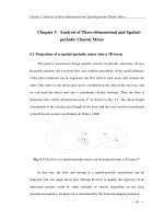
5.1 Projection of a spatial-periodic mixer into a 3D torus 89
5.2 A characterization method with one single mixer unit 90
5.2.1 Lyapunov exponent 90
5.2.2 Averaged dispersion rate of the mixer 93
5.2.3 The mechanism to analyze local mixing properties 96
5.2.4 Results and discussions 98

5.3 The mapping approach 102
— —
v
5.3.1 Methods to approximate the Poincaré map 104
5.3.2 Application to TLCCM-A 110
5.4 Conclusions 118
Chapter 6 Perturbed Rotating Flow and Chaotic Mixing

6.1 Analysis of the partial chaotic mixer 119
6.1.1 A rotating flow with intermittent perturbation 119
6.1.2 Observation of periodic and chaotic flow behaviors 122
6.1.3 The transition to chaotic flow 126
6.2 TLCCM-B — two interacting rotating flows 128
6.3 Numerical experiments on two-coupled rotating flows 130
6.3.1 Definition of the flow system 130
6.3.2 Numerical experiments 131
6.4 Some discussion on 3D steady and 2D unsteady chaotic flow 137
6.5 Conclusions 140
Chapter 7 Reynolds Number and Geometrical Effects on Passive
Chaotic Mixing
7.1 Influence of the fluid inertial effects on chaotic mixing 141
7.1.1 Performance of a 3D serpentine mixer at different Re 141
7.1.2 Reversible mixing in a co-joined 3D serpentine channel 146
7.2 Geometrical influences on passive chaotic mixing 149
7.2.1 Elimination of isolated regions through reorientation of fluids 149
7.2.2 Improved mixing in microchannel with grooved surface 154
7.2.3 Optimization of SHM mixer 160
— —
vi
7.3 Conclusions 164

Chapter 8 Conclusions and Recommendations
8.1 Conclusions 167
8.2 Recommendations 170
References
173

Appendix A Experimental Apparatus 191
Appendix B CO
2
Laser Processing of PMMA 192
Appendix C A Compact TLCCM Mixer 196
— —
vii
Summary
Microfluidics technology has received intensive attention in recent years due to
its wide applications in biological and chemical systems. One major issue is to mix
fluids at microscopic scales. In micro-geometries, the fluid viscous effect becomes
dominant, and micro flow typically falls in the laminar regime. In the absence of
turbulence, the fluid mixing becomes purely dependent on diffusion, which is a slow
molecular process. On the other hand, in many biological and chemical processes, fast
and complete mixing of relevant fluids is of crucial importance. The mixing quality
may determine the performance of the whole microfluidic system. In order to meet
the mixing requirements, various micromixers have been reported. Active mixers can
provide efficient mixing, but involve moving parts and external resources. For passive
mixers, many previous designs exhibit dependence on the fluid inertial effects and
only work well at relatively higher Reynolds number range. Up to date, micro fluid
mixing remains one of the most challenging problems and needs further exploration.
In this work, we have studied new passive micromixer design using the chaotic
advection mechanism. Novel designs have been developed. The models consist of two
branch microchannels that intermittently overlap and interlink across each other.

While the fluids are driven through the channel, rapid chaotic mixing can be achieved
through the repeated stretching and folding, splitting and recombination process. One
apparent advantage of the design is its independence of the fluid inertial effects. Rapid
mixing can be achieved even at extremely low Reynolds numbers (Re<<1). This
capability makes it very suitable for microfluidic applications, especially for mixing at
low flow rates and for highly viscous organic fluids. The two-layer structure of the
— —
viii
mixer can also be easily realized with commonly accessible fabrication techniques.
Relevant experimental testing has confirmed the effectiveness of the design.
To find out the influence of the fluid inertial force and the geometrical effects
on passive chaotic mixing, different configurations were studied including the 3D
serpentine channel, the channel with patterned grooves and the staggered herringbone
mixer (SHM). Relevant results show that, at low Re and near the linear Stokes flow
regime, the fluid mixing becomes reversible and rather difficult. At high Re when the
fluid inertial effects are important, the wandering channels can lead to recirculation
flow which favors the mixing. It is also found that the mixer with simple regular
structures may result in partial chaos where unmixed zones exist. In this situation, a
proper reorientation of the channel may reorganize the flow and eliminate the
invariant flow structures to achieve global mixing.
The chaotic mixing in a 3D microchannel was further analyzed using dynamical
tools. A characterization method and the mapping approach were proposed to evaluate
the spatial-periodic mixer. Relevant analysis only requires the flow field solution
within one single mixer unit. It greatly reduces the enormous work involved in 3D
CFD simulation. Numerical experiments were also performed using mathematically
modeled flow to reveal how chaotic mixing can be produced in perturbed rotating
flow system.
The current work includes both simulation and experimental study. Relevant
results will further our understanding of passive chaotic mixing in microchannels, and
provide valuable references for design and optimization of chaotic micromixers.

— —
ix
Nomenclature
Roman Letters
A Material interfacial area
C Species concentration
D Diffusivity
d Channel depth
De Dean number
D
h
Characteristic length
f Frequency
i, j, k Indices
L
D
Diffusion length
l Mixer length from inlet
Pe Péclet number
P Pressure
Q Flow rate
Re Reynolds number
R
c
Radius of curvature
r Radial coordinate, radius of supporting area
S Source
T Time period
t Physical time
u, v, w Velocity component in cartesian coordinates

V Fluid volume
x Transverse coordinate of the mixer cross section
y Longitudinal coordinate of the mixer cross section
— —
x
z The coordinate along the mixer length
Greek Alphabets
α
Aspect ratio
δ
Separation between two fluid particle trajectories
θ
Angular coordinate
λ
Lyapunov exponent
λ
′
Dispersion rate calculated within one mixer unit
v
Kinetic viscosity
ρ Density of the fluids
σ
,
σ
′
,
I
σ
Standard deviation
τ

Time delay for phase-space-reconstruction
Φ
(x, y) Fluid particle trajectory starting from point (x, y)
φ
Conserved quality per unit volume
ψ
Streamline function
Ω
Material interface/line based on particle-tracing simulation
Subscripts
On any variable Q:
Q
0
Initial value, upstream value
Q
N
Values at the N
th
mixer unit
Q
A
, Q
B
, Q
C
… Values at mixer cross section A, B, C…
— —
xi
List of Figures
Figure

Page

Fig. 1.1
Various stirring methods used for active micromixer design. 12

Fig. 1.2
Different designs of passive micromixer. 14

Fig. 1.3
Previously reported chaotic micromixers. 21


Fig. 2.1
Schematic illustration of the microchannel with grooved
surface. Relevant parameters:
c
w =1200,
c
d =450,
600==
sg
ww , 300=
g
d (unit:
m
µ
). The groove aspect
ratio:
α
=0.25.

27

Fig. 2.2
Cross-section velocity vector planes in the mixer with grooved
surface (view direction: facing the incoming flow).
28

Fig. 2.3
Mixing results in the microchannel with grooved surface at
Re=0.3,
α
=0.25. (a) Cross-sectional profiles of the
concentration. (b) Standard deviation versus the mixer length.
The coordinate
N
indicates the position of section
A
N
.
30

Fig. 2.4
Examples of particles trajectories in the mixer with grooved
surface at Re=0.3. The particles are released at the centre of
the two inlets. Please note that the vertical and horizontal axes
are drawn to different scales.
32

Fig. 2.5
Cross-sectional distribution of the colored particles along the

grooved mixer at Re=0.3
33

Fig. 2.6
Evolution of the material interface along the mixer at Re=0.3.
(a) Cross-sectional profile of the material interface at
A
10
and
A
20
. (b) Quantified results. The coordinate
N
indicates section
A
N
.
35

Fig. 2.7
Quantified mixing results in the grooved microchannel using
the particle-tracing method at Re=0.3.
37

Fig. 2.8
Schematic plot (a) and a photograph (b) of the experimental
setup for mixing test.
40

Fig. 2.9

The mixing picture in the microchannel with grooved surface
at Re=0.01
40



— —
xii
Fig. 3.1
Schematic illustration to show that chaotic mixing cannot be
produced in a 2D steady flow.
42

Fig. 3.2
Illustration of (a) stretching and folding; (b) stretching,
splitting and recombination process that commonly involved
in chaotic mixing
43

Fig. 3.3
Configuration of the TLCCM chaotic micromixer and relevant
parameters (unit:
m
µ
).
45

Fig. 3.4
Velocity vector planes of TLCCM-A at Re=0.2. The sections
are consistent with those indicated in Fig. 3.3(a).

47

Fig. 3.5
Velocity vector planes of TLCCM-B at Re=0.2. The sections
are consistent with those indicated in Fig. 3.3(b).
49

Fig. 3.6
Configuration of the 3D serpentine mixer. It also adopts a two-
layer structure and the depth of the channel is 150
m
µ
.
50

Fig. 3.7
Comparison of mixing results between TLCCM and the
serpentine mixer at Re=0.2. l indicates the mixer length. (a)
Mixing of the first 10 cycles of the serpentine mixer. (b)
Mixing in TLCCM-A. (c) Mixing in TLCCM-B. The
examined planes are A, B, C, D, etc., as indicated in Fig. 3.3.
52

Fig. 3.8
Quantified mixing results of TLCCM-A, B and the serpentine
mixer.
53

Fig. 3.9
Trajectories of examined inert particles (a) Model A, Re=0.2.

From (b.1) to (b.3), results of model B. (b.1) Re=0.2, particles
are released from the inlet centre. (b.2) Re=0.2, the particle is
released at the centre of section A. (b.3) Particles are released
at the same positions as that in (b.1) but at Re=60.
54

Fig. 3.10


Mixing results of TLCCM-A at Re=0.01, 1, 10 and 60. For
calculation of
'
σ
, the cross section of the mixer is divided into
17
×
12 sub-cells.
56

Fig. 3.11
In TLCCM-A, the standard deviation decreases exponential
fast along mixer length, Re=0.2.
N
stands for mixer units.
57

Fig. 3.12
Mixing results of TLCCM-B at Re=0.2, 10 and 60. (a) Cross-
sectional distribution of the particles. (b) Quantified mixing
results.

58

Fig. 3.13
Stretching of the material interface in TLCCM-A. (a) Particles
located near the material interface at Re=0.2. (b) Quantified
results versus Re.
60

Fig. 3.14
Stretching of the material interface in TLCCM-B. 60

— —
xiii


Fig. 4.1
Fabrication of meso-size mixer models for preliminary
experimental testing.
67

Fig. 4.2
Picture of TLCCM-B made of PMMA. 67

Fig. 4.3
Mixing results at Re=1 in: (a) a planar rectangular channel,
and (b) a 3D serpentine channel.
68

Fig. 4.4
Experimental mixing results of the TLCCM mixer at Re=0.01. 69

Fig. 4.5
Microchannels fabricated using CO
2
laser. (a) Cross-sectional
profile of a microchannel. (b.1) and (b.2) show the top-layer
and base-layer structure of the TLCCM mixer.
72

Fig. 4.6
Photographs of the PMMA micromixers TLCCM-A and
TLCCM-B; and the microstructures of the two-layer flow
channels after thermal bonding.
74

Fig. 4.7
Bonding strength test for solvent-assisted thermal bonding. 75

Fig. 4.8
Schematic of leakage test of thermally bonded microfluidic
mixer.
76

Fig. 4.9
Experimental mixing results of the TLCCM mixer at Re ~
0.01. The dashed lines in subfigures (a.1) and (a.2) indicate
the positions of the observation windows. Shadowed regions
indicate the top-layer channel.
77

Fig. 4.10
Fabrication process of PDMS mixer. 78

Fig. 4.11
Microphotographs showing a part of (a) the mould, and (b) the
cast microchannel of TLCCM-B.
79

Fig. 4.12
Mixing pictures of PDMS mixer at Re
≈
0.05. (a) TLCCM-A.
The dashed rectangles indicate the positions of the observation
windows. (b) TLCCM-B. The sample windows are consistent
with that in Fig.4.9 (a.2).
80

Fig. 4.13
Mixing results of TLCCM-A using chemical method. 85

Fig. 4.14
Mixing results of TLCCM-B using chemical method. 88



Fig. 5.1
The flow in a spatial-periodic mixer can be projected onto a
3D torus
T
3

.
89

Fig. 5.2
The definition of Poincaré section and the separation (
δ
)
between two particle trajectories in a spatial-periodic mixer.
91

— —
xiv
Fig. 5.3
Particle trajectories
)135 ,100(
Φ
and )150 ,100(
Φ
in TLCCM-
A at Re = 0.2. (a) 3D view. (b) The separation )(z
δ
versus the
mixer length. The saturation length is
≈
1.6 mixer units (4.07
mm).
93

Fig. 5.4
Averaged dispersion rate in the TLCCM mixer at different Re. 95

Fig. 5.5
Comparison of the standard deviation versus mixer length
between TLCCM-A and TLCCM-B at Re=0.2.
96

Fig. 5.6
Schematic illustration that
λ
′
-map together with the 2D
mapping information can be used to analyze the chaotic
dynamics and mixing performance of time-independent
spatial-periodic chaotic micromixer.
97

Fig. 5.7
Results of mixer TLCCM-A. (a.1) '
λ
-map, and (a.2) cross-
sectional moving behavior of the fluid particles within one
mixer unit at Re=0.2. The arrows point the moving direction,
and the length correspond to the distance the particles have
traveled. (b) '
λ
-map at Re=10. (c) '
λ
-map at Re=60.
99

Fig. 5.8
The configuration of a partial-chaotic micromixer. Its
geometrical parameters are consistent with that of the TLCCM
mixer.
99

Fig. 5.9
Results of a partial-chaotic mixer. (a) '
λ
-map,
and (b)
cross-
sectional moving behavior of the fluid particles within one
mixer cycle at Re=0.2.
100

Fig. 5.10
Mixing results of the partial chaotic mixer. (a) Simulation
results at Re=0.2. (b) Experimental mixing picture at Re=0.01.
101

Fig. 5.11
Results of TLCCM-B. '
λ
-map (left figure), and cross-
sectional moving behavior of the particles within one mixer
unit (right figure). (a) Re=0.2. (b) Re=60.
102

Fig. 5.12

Triangular weighted interpolation scheme.
105

Fig. 5.13
Local Shepard method. 106

Fig. 5.14
Point distribution for mapping approach (Mesh 1, 11222
points).
110

Fig. 5.15
Weighted least-square polynomial fitting (a) before and (b)
after improvement. (о): supporting points. (●): interpolating
point, and its exact position on the next plane. (□): the
mapping position. Data are from TLCCM-A, Re=0.2.
112

Fig. 5.16
Schematic of selection of supporting points. 113

— —
xv
Fig. 5.17
Distribution of
Err
(a) before and (b) after improvement.
Results of TLCCM-A, Re=0.2 using Mesh 1.
113

Fig. 5.18
Root mean square of the errors versus mesh size. Comparison
of WLS-PF (w
1
) with Tri-WI and Shepard’s method.
114

Fig. 5.19
Root mean square of the errors versus mesh size for WLS-PF
method using different weighting functions.
114

Fig. 5.20
(a) Comparison of the cross-sectional mixing in TLCCM-A, at
Re=0.2. Right figures are results using WLS-PF (
1
w
) mapping
method with Mesh 1. Left figures are obtained using particle-
tracing method in CFD study. (b) Comparison of the
quantified mixing results among the three mapping schemes
(with Mesh 1) and the particle-tracing method.
117

Fig. 5.21
Relative error on the standard deviation of the concentration
realrealmap
σσσ
′′
−

′
/ versus the number of mesh points.
117



Fig. 6.1
Evolution of examined fluid material lines as shown in section
A
0
.
L
0
is the mixer unit-length,
mL
µ
4.636
0
≈ . The circular
material lines are respectively R=20, 30, 50 and 80
m
µ
,
centered at (46, 150) (
m
µ
). A black point is placed at the red
cycle to illustrate the rotation.
121

Fig. 6.2


(a) The cross-sectional mixing after 10 mixer units. (b) The
points selected for phase portrait reconstruction.
124

Fig. 6.3
Reconstructed phase-portraits using [ )](),(),(
dzzxzyzx
+
.
They correspond to: (a) Period-1 point (41.5, 148). (b) Period-
3 point (90.6, 165.9). (c) Point (24, 130) near the edge of the
stable region. (d) Point (17, 123) in the chaotic area.
125

Fig. 6.4
Divergence of neighboring particle trajectories in the partial
chaotic mixer.
126

Fig. 6.5
Evolution of examined fluid particles in TLCCM-B at Re=0.2.
Their initial distribution is shown in section
A
0
. The radii of
the circles are respectively R=10, 25 and 50, centered at (-80,
85) and (62, 152) (

m
µ
).
128

Fig. 6.6
(a) Distribution of period-1 (indicated by “o”), period-3 (“
∆
”)
and a chaotic (“
×
”) point. (b) ~ (d): Reconstructed phase-
portraits of the trajectories at point (61.5, 152), (44.7, 146.7)
and (-5, 125).
129

Fig. 6.7
Schematic diagram of two coupled rotation flows. 131

— —
xvi
Fig. 6.8
Influence of time interval
T
on chaotic mixing,
0
r
=0.5,
a
π

0.1
=
. The Poincaré sections are created by tracing 10
particles distributed along the
x
-axis at
x=
001.0
±
, 05.0
±
,
1.0
±
, 15.0
±
and 2.0
±
.
132

Fig. 6.9
Particle trajectories at (a) point (0.5
r
0
, 0
0
) and (b) point (0.5
r
0

,
-30
0
) with respect to
o
1
. Parameters are:
a
π
0.1
=
,
T
=1.
134

Fig. 6.10
Poincaré section created by tracing point (0.5
r
0
, -30
0
) (point 0
in Fig.6.9 (b)) with respect to
o
1
within in
t
=10000. (a)
a

π
0.1
=
,
T
=1. (b)
a
π
5.1
=
,
T
=1.
135

Fig. 6.11
Exponential divergence between trajectory pair )0 ,001.0(
−
Φ

and )0 ,001.0(
Φ
at
a
=
π
5.1 ,
T
=1,
0

r =0.5
.
135

Fig. 6.12
Mixing in the coupled rotation flow system at
a
π
5.1
=
,
T
=1.
The initial material blobs are 0.2
×
0.2 and centered at
o
1
(-
0.25, 0), and
o
2
(0.25, 0).
136

Fig. 6.13

Mixing in the coupled rotation flow system at
a
π

5.1
=
,
T
=1.
The initial material blobs are 0.2
×
0.2 and centered at
o
1

( 20.0
−
, 0), and
o
2
(0.20, 0),
r
0
=0.5.
137

Fig. 6.14
Cross-sectional streamlines

near section
A
(see Fig. 5.8)

in the

partial chaotic mixer.
z
A
stands for the position of section
A

(unit:
m
µ
).
139



Fig. 7.1
The reference coordinate system of the 3D serpentine mixer
(unit:
m
µ
). The shadow area indicates the “
C
-shaped” blocks
in the top layer.
141

Fig. 7.2
Velocity vector planes of the 3D serpentine mixer at Re=0.2
and 60.
142

Fig. 7.3
Examples of

fluid particle trajectories at different Re. The
particles are released from
P
1
and
P
2
at section
A
as shown in
Fig.7.1. In (b) & (c), the 3D trajectories are projected onto the
x-y
plane.
144

Fig. 7.4
(a) & (b)
λ
′
-
map of the serpentine mixer at Re=0.2 and 60.
(c) Averaged dispersion rate versus Re.
144

Fig. 7.5
Mixing results of the 3D serpentine mixer at different Re. (a)
Cross-sectional distribution of the inert particles. (b) Standard

deviation versus the mixer length (
N
indicates section
A
N
).

145

Fig. 7.6
Configuration of the mixer that demonstrates reversible
mixing at low Re (Parameters unit:
m
µ
).
147

— —
xvii
Fig. 7.7
Mixing in the co-joined serpentine mixer at Re=0.2. (a)

Reversible fluid mixing. (b) Particle trajectories showing the
regularity of the flow.
148

Fig. 7.8
λ
′
-

map of the mixer using co-joined serpentine channel, near-
zero
λ
′
indicates the stable property of the system.
149

Fig. 7.9
Experimental results in the co-joined serpentine channel at
Re=0.2. Applied fluid is 98% glycerol-2% food dye solution.

149

Fig. 7.10
TLCCM-B and the improved models. The shadow area
indicates the top-layer channel. The distance between
neighboring knot positions is defined as 1( m 636
µ
≈
). Other
parameters are consistent with TLCCM-B.
152

Fig. 7.11
Projection results of the trajectories
Φ
(-81.6, 88.8) and
Φ
(61.5, 152) (
m

µ
) in the
x-y
plane. M1, Re=0.2.
152

Fig. 7.12
Distribution of the fluid elements in successive mixer planes
in M1 at Re=0.2.
152

Fig. 7.13
Comparison

of the

mixing results between TLCCM-B and the
improved models.
154

Fig. 7.14
Microchannel with grooved surface and the reference
coordinates. The shadow area indicates the grooves. (a) Model
A. (b) Model B.
155

Fig. 7.15
Channel length needed to complete one circulation in model
A.
156

Fig. 7.16
Velocity vector planes of model B at Re=0.3,
α
=0.33. The
sections are consistent with those indicated in figure 7.14.
157

Fig. 7.17
3D and 2D plots

of some trajectories in (a)

model A; and (b)
model B at Re=0.3,
α
=0.33. The particles are released at the
centre of inlet 1 and inlet 2.
157

Fig. 7.18
Mixing results in the microchannel with grooved surface at
Re=0.3. (a) Model A, 33.0
=
α
. (b) Model B, 33.0
=
α
. The
cross sections are as indicated in Fig. 7.14(b). (c) Quantified

mixing results.
158

Fig. 7.19
Experimental mixing pictures in grooved channel at Re=0.01.
The applied fluid is 98% glycerol-2% food dye solution.
159

Fig. 7.20
Schematic structure of the SHM mixer. The shadow area
indicates the patterned grooves. In the original model (a) (for
case 1 and case 2), one cycle includes 20 grooves. In the
modified model (b) (for case 3),
α
is increased to 0.33, and
161

— —
xviii

g
N
is reduced to 4.
Fig. 7.21
Mixing results of SHM at Re=0.2. From top to bottom in both
(a) & (b), the pictures are respectively for case 1, 2 and 3. (a)
The plane is examined at the mid-height of the main channel.
(b) The cross-sections are indicated by the dashed lines in
figure (a). (c) Standard deviation versus the mixer length.
162

Fig. 7.22
Experimental mixing pictures in SHM at Re~0.01. 164



Fig. A.1


Experimental apparatus for mixing test of PDMS microfluidic
mixer.
191

Fig. B.1
The CO
2

Laser system used to fabricate the PMMA mixers. 192

Fig. B.2
Cross-section profile of a microchannel cut by CO
2
laser. 193

Fig. B.3
Width/ depth of the channel versus the feeding rate. The
PWM duty cycle is 50%,
p
N
=2.

193

Fig. B.4
Width/ depth of the channel versus the PWM duty cycle. The
feeding rate is 15 cm/s,
p
N
=2.
193

Fig. B.5
Channel width/ depth versus the feeding rate when three
overlapping laser beams are applied. The spacing is 80
m
µ
,
PWM=50%,
p
N
=2.
194

Fig. B.6
Channel width/depth versus the beam spacing. The feeding
rate is 25 cm/s, PWM=50%,
p
N
=2.
195

Fig. C.1
A compact TLCCM mixer with multi-layer structures. 197

Fig. C.2
Cross-sectional mixing results observed using particle-tracing
simulation. The positions of the cross sections are indicated in
Fig. C.1(b).
198

Fig. C.3
Standard deviation versus the mixer length.

The 0-point
corresponds to location 1 as indicated in Fig. C.1(b). The
distance between plane 1 and 2 is defined as 2 (the vertical
depth between different layers is not taken into account).
199

Fig. C.4
Experimental mixing picture at Re~0.01. The rapid reduction
in the fluid striation thickness suggests good mixing. (Note:
The device tested here only contains one layer of the channel.)
199


— —
xix


List of Tables

Tab. 3.1


Pressure loss at different Re for TLCCM and 3D serpentine
mixer.
61

Tab. 6.1
Axial gradient of velocity
w
at transient attracting/repelling
point
P
Q
.
139

Tab. B.1
Influence of number of passes on channel geometry. 194


Chapter 1 Introduction

— —
1

Chapter 1 Introduction
1.1 A brief retrospect on fluid mixing study
1.1.1 Mixing and its applications

Mixing is present in many fields, from the food, pharmaceutical, chemical and
environmental industries to our daily life. Roughly speaking, mixing means the
stirring of initially separated substances to increase the homogeneity. It may be either
a pure physical change, or a chemical change which involves the reduction of
reactants and the formation of new products (Nagata, 1975).
Based on the phase of the constituents to be mixed, there are different mixing
problems (Nagata, 1975; Oldshue, 1983; Paul, 2003; etc.) which can be categorized
into four regimes: (1) Solid-solid mixing. In pharmaceutical production, catalyst
preparation, and food industry, it usually requires the mixing of granular particles.
This can be achieved with rotating drum blender, rotary mixer, etc. (2) Solid-liquid
mixing. It may be encountered in crystallization operation or solid catalyzed liquid
reactions. This problem involves the suspension and distribution of solid particles in
liquid. (3) Gas-liquid mixing. In some processes, such as oxidation and biological
fermentation, the contacting between gases and liquids is important. It requires the
distribution of small bubbles in a liquid. (4) Liquid-liquid mixing. For immiscible
fluids, it means the formation of dispersed small droplets of one fluid inside another.
For miscible fluids, besides the reduction in the length scale of fluid elements, it also
involves molecular mixing to change the concentration to obtain homogeneity.
Chapter 1 Introduction

— —
2

Mixing is a central concern in many industrial processes (Harnby et al., 1992).
For example, in chemical production, the yield and quality of the final products are
mainly determined by the mixing efficiency of the reactants. In assays operations, fast
and complete mixing of the reagent with the sample can greatly reduce the total
analysis time and improve the detection sensitivity. Fast mixing between the fuel and
air is required for efficient and complete combustion. Conversely, poor mixing may
cause severe problems, such as increased production cost, excessive analysis time,

and wasteful inefficient combustion. Besides these examples, mixing is also an
important issue in crystallization, fermentation and polymer processing, etc.
1.1.2 Fluid mixing mechanisms and traditional mixing devices
Even though mixing is so important and used everywhere, it has evolved as a
scientific discipline only from around the 1950s (Paul et al., 2003). Due to its
diversity in applications, early studies on mixing were mainly on a case-by-case basis.
Relevant discussions can be found in Uhl & Gray (1966), Nagata (1975), Oldshue
(1983), and Ottino (1989).
In the current study, we have mainly investigated the fluid mixing problem.
Basically, fluid mixing involves the reduction in the length scales of the bulk fluid
elements. For chemical reactions between miscible fluids, the reactants must be mixed
to a molecular level before reactions can occur. This is achieved through molecular
diffusion, which is the final step of mixing. Diffusive mixing is characterized by the
molecular diffusivity. The volume of mixed fluids can be expressed as
DtAV =
(1.1)
where
A
is the contact area between the fluids,
D
is the molecular diffusivity,
t
is time.
Chapter 1 Introduction

— —
3

Diffusion is usually a very slow process. It becomes significant only after the bulk
fluid elements are reduced into much smaller scales, or when the material interface is

greatly increased. Efficient mixing usually requires the stretching and folding of fluids,
and may also involve the breakup process. Depending on the flow conditions, fluid
mixing exhibits following characteristics.
(1) Turbulent mixing.
It is well known that turbulent flow that occurs at high Reynolds numbers
favors mixing. The physical meaning of Re is the ratio of the fluid inertial forces over
the viscous forces. High Re means less friction and low cost of fluid stirring. A
turbulent flow is characterized by eddies of various size, and exhibits unsteady,
disorder and random behaviors. These eddies cause rapid dispersion of fluids, which
is called eddy diffusion or turbulent diffusion. More discussions can be found in
Chaté et al. (1999).
(2) Laminar mixing.
At low Re, the fluid viscous effects become significant leading to laminar flow.
Turbulent mixing is no longer available. In an intermediate regime at around Re ~ 100,
the fluid inertial effect may still be important while the flow is laminar. Vortices may
occur (e.g. in the Dean flow) and improve the mixing. At lower Re where the inertial
forces become negligible, the mixing will become more difficult. In order to meet the
mixing requirements, some stirring strategies are usually required to promote mixing.
The stirred tank or vessel is one of the most commonly used mixing devices. It
is involved in over 50% chemical productions worldwide (Paul et al., 2003). In the
tank, an impeller is applied for mechanical agitations. Depending on the impeller
Reynolds number, it may work under either laminar or turbulent flow conditions. So
Chapter 1 Introduction

— —
4

far, there have been numerous reports on this subject, including the mixing quality
analysis (Metzner & Taylor, 1960; Tatterson, 1991; Guillard et al., 2000; Alvarez et
al., 2002a, 2002b), impeller design to maximize the mixing efficiency (Dickey et al.,

2001; Szalai et al., 2004; Kumaresan & Joshi, 2006; Aubin & Xuereb, 2006),
numerical and experimental studies (Yoon et al., 2001; Li et al., 2005; Hartmann et al.,
2006), etc.
Besides the stirred tank or vessel, in-line mixers have been widely used in
industries. These include the static Kenics mixer (Bakker & LaRoche, 1993; Hobbs &
Muzzio, 1997, 1998a, 1998b), SMX
TM
mixer (Zalc et al., 2002, 2003), and the
impinging jet mixer (Scampavia et al., 1995; Andreev et al., 1999.), etc. The Kenics
mixer consists of a series of right- and left-handed helical elements connected with a
90
o
rotation. For the SMX mixer, it contains intersecting guide bars that are welded
together. Both the mixing elements are mounted in a cylindrical pipe. They can
continuously split, redirect and recombine the streams to increase the homogeneity.
For the jet mixer, it uses a jet flow to cause the entrainment of ambient fluids to
achieve fast mixing. While the mixing tanks are mainly used for batch production,
these mixers do not involve moving parts and can be applied for continuous operation.
1.2 New issue — fluid mixing at micro scales
1.2.1 Microfluidics and the need of micro fluid mixing
1.2.1.1 Development of the microfluidics technology
The advent of microfluidics has benefited from the progress in the micro-
analytical methods and microfabrication technology (Whitesides, 2006). One
Chapter 1 Introduction

— —
5

motivation is the development of the micro-total-analytical systems (
TAS

−
µ
) which
has made it possible to achieve high resolution and sensitivity using very small
amount of samples. The second one is the development of microelectromechanical
systems (MEMS), because the photolithographic processes for forming
microstructures in silicon substrates are usually used for fabrication of microfluidic
devices (Verpoorte & Rooij, 2003). Today, alternative micromachining techniques
such as laser-ablation, injection moulding, hot-embossing, etc. are increasingly
applied using polymer materials. Microfluidic technology has wide applications for
biological and chemical processes, including genetic analysis, disease diagnosis, drug
delivery and chemical synthesis, etc.

In recent years, there has raised intensive
research on a verity of topics such as fabrication techniques, individual microfluidic
component design, system integration and applications (Liu & Grodzinski, 2003; Ng
et al., 2002), etc. Since its advent, the microfluidics has seen rapid progress.
Comprehensive reviews in this field were presented by Stone et al. (2001; 2004),
Beebe et al. (2002) and Whitesides (2006).


Microfluidic components for fluid manipulations include microchannel,
micropump, microvalve, micromixer and microfilter, etc. These individual functional
devices can be integrated into a system to perform certain analytical or processing
tasks. It is called lab-on-chip (LOC) (Figeys & Pinto, 2000), or
µ
-TAS (Manz et al.,
1990; Reyes et al., 2002; Auroux et al., 2002). With respect to biological applications,
similar terms for the conception include bio-MEMS and bio-chips (DNA-Chip, RNA-
Chip, Protein-Chip, etc.). These microsystems provide a convenient way for various

biological processes. They may be fabricated with silicon, glass or polymer materials.
All the steps for bio-chemical analysis, including sample injection, mixing, reaction