Fluid mixing enhancement through chaotic advection in mini micro channel 3
Bạn đang xem bản rút gọn của tài liệu. Xem và tải ngay bản đầy đủ của tài liệu tại đây (10 MB, 78 trang )
Chapter 5 Analysis of Three-dimensional and Spatial-periodic Chaotic Mixer
— —
89
Chapter 5 Analysis of Three-dimensional and Spatial-
periodic Chaotic Mixer
5.1 Projection of a spatial-periodic mixer into a 3D torus
The passive micromixer design usually consists of periodic structures. At low
Reynolds numbers, the involved flow also exhibits periodicity. If the small influence
of the inlet conditions can be neglected, the flow field in each mixer unit remains the
same. The outlet of one mixer unit can be considered as the inlet of the next one, and
we can bend the mixer unit into a continuous circular structure. Thus the flow is
projected onto a three dimensional torus T
3
as shown in Fig. 5.1. The mixer length
corresponds to the circular axial length of the torus and the cross-section corresponds
to the Poincaré section (see Doherty & Ottino, 1988).
P
2
P
1
Fig. 5.1 The flow in a spatial-periodic mixer can be projected onto a 3D torus T
3
.
In this way, the flow and mixing in a spatial-periodic micromixer can be
analyzed with one single mixer unit. Though the flow is regular, the trajectory of an
individual particle could be either periodic or chaotic depending on the local
dynamical properties. Its behavior is determined by the Poincaré mapping function.
Chapter 5 Analysis of Three-dimensional and Spatial-periodic Chaotic Mixer
— —
90
5.2 A characterization method with one single mixer unit
1
5.2.1 Lyapunov exponent
Lyapunov exponent (
λ
) is an important parameter for distinguishing various
chaotic systems. It measures the exponential rate of divergence between two initially
neighboring orbits. Positive
λ
is one signature of chaos, where the nearby trajectories
diverge exponentially fast. Zero
λ
indicates stable systems which exhibit Lyapunov
stability. The negative
λ
is the characteristic of dissipative systems which exhibit
asymptotic stability. In a flow system, the value of
λ
can be measured from the
separation between nearby fluid particles. Its magnitude reflects the stretching rate or
how fast a concentrated solute/dye is transported into the fluid domain. In Niu and
Lee’s (2003) study, Lyapunov exponent was used as a mixing index to evaluate the
chaotic behavior of their mixer. In Aubin et al.’s (2003) study, they also discussed the
application of this parameter as a criterion to quantify the mixing. The Lyapunov
exponent is usually calculated as
=
∞→
)0(
)(
ln
1
lim
δ
δ
λ
t
t
t
(5.1)
where )0(
δ
is the initial separation of two close trajectories in a phase plane and )(t
δ
is the separation at time t.
For a passive mixer consisting of periodic structures, it involves a time-
independent open flow. To calculate
λ
, the separation between particle trajectories is
projected onto one mixer cross-section, i.e. Poincaré section (x-y plane) at each mixer
1
The characterization method is included in our paper: Xia HM, Shu C, Wan S, Chew YT. 2006.
Influence of Reynolds number on chaotic mixing in spatially periodic micromixer and its
characterization using dynamical system techniques. J. Micromech. Microeng., 16, 53.
Chapter 5 Analysis of Three-dimensional and Spatial-periodic Chaotic Mixer
— —
91
unit. Suppose that two initially close inert particles are released at the inlet. As they
move downstream, their trajectories (streamlines) successively intersect with the
Poincaré sections. Their separations )(z
δ
can be recorded (as shown in Fig. 5.2).
Then the Lyapunov exponent
λ
is calculated by
∑
−
=
+
∞→
=
1
0
1
)(
)(
ln
1
lim
N
i
i
i
N
z
z
N
δ
δ
λ
(5.2)
where )(z
i
δ
is the separation between the particle trajectories at the sampled cross-
section of the
th
i mixer unit. It is a function of the mixer length
z
(or the number of
the mixer unit
i
).
Fig. 5.2 The definition of Poincaré section and the separation (
δ
) between two
particle trajectories in a spatial-periodic mixer.
Usually,
λ
is calculated after iteration of many mixer units. However, in
numerical studies, it involves new problems. Since the evolution of the particle
trajectories is based on the discrete flow field solution, it is reasonable to set the initial
separation )0(
o
δ
comparable with the computational mesh size. In such a situation,
according to our studies, the saturation length may soon be reached. That is, the
particle separation )(
z
N
δ
has increased to a scale comparable with the dimension of
the mixer cross section. Afterwards it only exhibits some kind of oscillation but will
Chapter 5 Analysis of Three-dimensional and Spatial-periodic Chaotic Mixer
— —
92
no longer increase.
One example is given in Fig. 5.3. The results are for mixer TLCCM-A at Re 0.2.
Two inert particles are released at
P
a
(100, 135) and
P
b
(100, 150) (
m
µ
) in section
A
0
(the reference coordinates are shown in Fig. 5.2). The initial separation is
m
µδ
15)0(
0
= . The 3D view of the trajectories (expressed as )(
a
P
Φ and ))(
b
P
Φ is
illustrated in Figure 5.3(a). Figure 5.3(b) plots the separation as a function of the
mixer length, which is translated into the number of mixer units (per mixer unit length
is
≈
2.546
mm
). It shows that within 1.6 mixer-unit length, the trajectories diverge
roughly exponentially by
NoN
e
72.1
⋅≈
δδ
.
Positive
λ
indicates the occurrence of chaotic advection. After that, the
distance in the plane between the particles has increased to
)15( m)( 235
06.172.10
me
s
µδµδδ
==⋅≈
×
.
This value is comparable with the dimension of the Poincaré section (cross section of
the mixer) which is 424.3
×
300 (
m
µ
). Afterwards,
δ
shows no further increase. The
Lyapunov exponent
λ
should be calculated within the saturation length, which is
hard to predict as it depends on different mixer designs and the local dynamical
properties of the flow.
Chapter 5 Analysis of Three-dimensional and Spatial-periodic Chaotic Mixer
— —
93
(a)
0 1 2 3 4
-1
0
1
2
3
4
(1.6, 2.75)
Ln (δ(z)/ δ(0))
mixer length (N)
(b)
Fig. 5.3 Particle trajectories )135 ,100(
Φ
and )150 ,100(
Φ
(
m
µ
) in TLCCM-A at
Re = 0.2. (a) 3D view. (b) The separation )(z
δ
versus the mixer length. The
saturation length is
≈
1.6 mixer units (4.07 mm).
5.2.2 Averaged dispersion rate of the mixer
As mentioned in Section 5.1, for a spatially periodic mixer, its flow field
solution in each mixer unit stays invariant. It contains all the information of the flow
in the whole mixer system. It might not be necessary to calculate
λ
after many mixer
units as defined by Eq. (5.2) to analyze the dynamical properties of the flow.
Here we propose a method to characterize mixers consisting of spatial-periodic
structure. Firstly, the divergence rate between neighboring particles is calculated
within one single mixer cycle. Suppose that a pair of particles is released at (
1,i
x ,
1,i
y )
Chapter 5 Analysis of Three-dimensional and Spatial-periodic Chaotic Mixer
— —
94
and (
2,i
x ,
2,i
y ) in a mixer cross-section
N
A . The initial separation is
N
i
δ
. After one
mixer cycle, their separation becomes
1+N
i
δ
on section
1+N
A . Then, the divergence
rate within one mixer cycle at
i
λ
′
is calculated as
N
i
N
i
i
yx
δ
δ
λ
1
ln),(
+
=
′
. (5.3)
For fair comparison among different mixers of various unit-lengths,
λ
′
can be
calculated over a same distance L. L is not limited to one mixer cycle, but it should be
within the saturation length. Another issue involved is the choice of the initial
separation
N
δ
. In numerical studies, it can be set close to the computational mesh
size. Our testing shows that within a wide range of
N
δ
,
λ
′
remains quite constant.
Secondly,
λ
′
is a function of the position (x, y) in section
N
A . Many particle pairs
should be examined with an attempt to cover the whole flow region. For each particle
pair, it corresponds to a value of
i
λ
′
which is assigned to
]2/)( ,2/)[(
2,1,2,1, iiii
yyxx ++
. A collection or set of
/
i
λ
(
=
i
1, 2 …k) will reflect the
complete information of the whole mixer. To facilitate the analysis,
i
λ
′
is plotted over
section
N
A , which is termed here as
λ
′
-map. The averaged value
∑
=
′
=
′
k
i
i
k
1
)1(
λλ
over the plane reflects the overall chaotic level of the flow. It measures the ability of a
mixer to disperse concentrated species into other flow domain.
We applied this method to examine the current TLCCM mixer. The two models
have similar structures, and the mixer unit-length of model B is one half that of model
A. For comparison, the results of model B are calculated within 2-mixer-units length.
Relevant results are plotted in Fig. 5.4. It is found that: (1) In both models, the
Chapter 5 Analysis of Three-dimensional and Spatial-periodic Chaotic Mixer
— —
95
positive
λ
′
indicates the occurrence of chaotic advection. (2) For model A and in the
Re range from 0.02 to 1, the value of
λ
′
remains rather constant at around 0.62. It is
just as expected since the flow characteristics retain invariant at Re<1. (3) For both
the mixers, in the moderate Re range, their chaotic properties are promoted with
increase of Re. For model A,
λ
′
increases to 0.97 at Re=10 and 1.69 at Re=60. For
model B, its value increases from 1.18 at Re=0.2 to 1.34 at Re=10, and it further
increases to 1.85 at Re=60. (4) It also shows that at Re=0.2, the value of
λ
′
in model
B is higher than that in model A. Actually as compared in Fig. 5.5, model B does
exhibit faster mixing than model A within a 10-mm mixer length. After that, mixing in
model A is slightly better. This is because while model A is globally chaotic, model B
contains both chaotic and stable zones where the mixing is very slow.
0.01 0.1 1 10 100
0.0
0.5
1.0
1.5
2.0
TLCCM-A
TLCCM-B
λ
'
Re
Fig. 5.4 Averaged dispersion rate in the TLCCM mixer at different Re.
All the above mentioned observations are quite consistent with the earlier
mixing results. This validates the application of
λ
′
as an index of the mixing
performance for partial-periodic mixer. However, while
λ
′
presents an overall
estimation of the mixing quality, it does not provide detailed information at a specific
Chapter 5 Analysis of Three-dimensional and Spatial-periodic Chaotic Mixer
— —
96
local region. For a mixer system, it may contain both chaotic and non-chaotic zones.
Further information is required to distinguish the local mixing properties.
0 2 4 6 8 10 12
0.0
0.1
0.2
0.3
0.4
0.5
σ
'
Mixer length (mm)
Fig. 5.5 Comparison of the standard deviation versus mixer length in TLCCM-A and
TLCCM-B at Re=0.2.
5.2.3 The mechanism to analyze local mixing properties
The Poincaré mapping is the additional information to characterize 3D periodic
mixers. It can be constructed within one mixer unit,
)]([)(
1 NN
APfAP
=
+
(5.4)
where )( AP is the set of all the particles’ positions on section
A
. Since the flow is
periodic, the
λ
′
-map and Poincaré mapping function over each mixer cycle are fixed.
If Eq. (5.4) is known, the mixing of fluids at successive Poincaré sections can be
directly predicted. Unfortunately, for a complex physical 3D flow, the specific
analytical description of the formula is usually not available.
To extract the mapping information, we may analyze the moving behaviors of
the particles on the Poincaré section. They provide useful information and facilitate
Chapter 5 Analysis of Three-dimensional and Spatial-periodic Chaotic Mixer
— —
97
relevant analysis. The mechanism to analyze the local mixing property includes the
combination of the mapping information and aforementioned
λ
′
-map results. The
method is illustrated in Fig. 5.6. (1) If
λ
′
as defined in Eq. (5.3) is generally positive
over the mixer cross section, it means that the mixer exhibits overall chaotic
properties. A blob of concentrated solute placed anywhere can eventually be dispersed
into the whole flow domain. (2) If the
λ
′
value is globally zero or close to zero, it
indicates a stable system. The concentrated solute will remain unmixed. (3) In a third
situation,
λ
′
is only positive in partial flow regions (labeled in Fig. 5.6 as region a);
and it is zero/near-zero in the rest of zones (region b). This case is a little more
complex, and we need to further check the Poincaré mapping information. First, if the
fluids in region b have been moved to region a within one mixer cycles, it means that
the concentrated fluids can be dispersed into the flow domain in the following mixer
cycles. So the mixer is still overall chaotic, and all the fluids can finally be well mixed.
Second, if the fluids are trapped in region b, then an isolated unmixed region would
form there. The mixer is only partially chaotic, and the mixing is incomplete.
Fig. 5.6 Schematic illustration that
λ
′
-map together with the 2D mapping information
can be used to analyze the chaotic dynamics and mixing performance of time-
independent spatial-periodic chaotic micromixer.
Chapter 5 Analysis of Three-dimensional and Spatial-periodic Chaotic Mixer
— —
98
5.2.4 Results and discussions
Three mixers were analyzed using current characterization method. Their results
and relevant discussions are presented below.
5.2.4.1 Results of TLCCM-A
The results of TLCCM-A are shown in Fig. 5.7. At Re = 0.2,
'
λ
is roughly
positive over the whole
x-y
plane. In the regions indicated as
1
a
and
2
a
, the
magnitude of '
λ
is relatively small, but Fig. 5.7(a.2) reveals that the fluids there move
towards their neighboring area where '
λ
is large. According to the analysis as
illustrated in Fig. 5.6, the regions near
1
a
and
2
a
are still chaotic. As confirmed by
previous observation, the fluids are mixed homogeneously. Figures 5.7(b) and 5.7(c)
show that the chaotic advection was promoted as Re increases to 10 and 60.
5.2.4.2 Results of a partial-chaotic mixer
The second mixer analyzed is shown in Fig. 5.8. It is similar to TLCCM-B but
with a simpler structure. The base-layer channel turns to the top-layer from only one
side of the mixer. Fig. 5.9 presents its results at Re=0.2. Analysis suggests that it is a
partially chaotic mixer. In region around
1
b
(subfigure (a)), '
λ
is near-zero. Subfigure
(b) reveals that nearby fluids are trapped there, i.e. after traveling one mixer unit, the
positions of particles on the
x-y
plane remain unchanged. Since the '
λ
-map repeats
itself in subsequent mixer cycles, an invariant isolated region would form near point
1
b
. The local fluids remain concentrated. Similar phenomena also exist in a smaller
area indicated by
2
b
, and the mixing there is slow.
Chapter 5 Analysis of Three-dimensional and Spatial-periodic Chaotic Mixer
— —
99
(a.1) (a.2)
(b) (c)
Fig. 5.7
Results of mixer TLCCM-A. (a.1) '
λ
-map, and (a.2) motion in the Poincaré
cross-section of the fluid particles within one mixer unit at Re=0.2. The arrows point
in the direction of motion, and the length correspond to the distance the particles have
traveled. (b) '
λ
-map at Re=10. (c) '
λ
-map at Re=60.
Fig. 5.8
The configuration of a partial-chaotic micromixer. Its geometrical parameters
are consistent with that of the TLCCM mixer.
Chapter 5 Analysis of Three-dimensional and Spatial-periodic Chaotic Mixer
— —
100
(a) (b)
Fig. 5.9
Results of a partial-chaotic mixer. (a) '
λ
-map;
(b)
cross-sectional moving
behavior of the fluid particles within one mixer cycle at Re=0.2.
These deductions are consistent with the mixing results as shown in Fig. 5.10.
Fig. 5.10(a) shows the cross-sectional mixing at Re=0.2. In the left-lower corner,
there is a large dead flow zone. For the rest of the region, a small stable island is
embedded in a chaotic area. Fig. 5.10(b) is the experimental mixing picture at Re =
0.01. The mixing is apparently incomplete. While mixing occurs on one side of the
mixer, the fluids on the other side remain concentrated and cannot be transported into
the other flow field. Obviously this isolated region always exists. This agrees well
with above-mentioned analysis that at low Re this mixer is only partially chaotic. The
analysis provides some guidance for improvement. To reduce the isolated regions, the
geometry of the left side channel should be changed to introduce more stirrings in the
fluids.
Chapter 5 Analysis of Three-dimensional and Spatial-periodic Chaotic Mixer
— —
101
(a)
(b)
Fig. 5.10
Mixing results of the partial chaotic mixer. (a) Simulation results at Re=0.2.
(b) Experimental mixing picture at Re=0.01.
5.2.4.3 Results of TLCCM-B
Actually, TLCCM-B can be considered as an improved model of the above-
analyzed partial-chaotic mixer. Its results are demonstrated in Fig. 5.11. At Re=0.2,
the flow near the locations indicated at
c
1
and
c
2
is quite stable. In comparison with
the partial-chaotic mixer, as more stirrings are induced through rotating the flow from
the base-layer channel to the top-layer, the stable region near
c
1
is greatly reduced.
This reflects the influence of geometry complexity on passive mixing. At Re=60, the
flow becomes much more chaotic. The originally unmixed zones are eliminated. The
analysis also agrees well with the corresponding mixing results.
Chapter 5 Analysis of Three-dimensional and Spatial-periodic Chaotic Mixer
— —
102
(a)
(b)
Fig. 5.11
Results of TLCCM-B. '
λ
-map (left figure), and cross-sectional moving
behavior of the particles within one mixer unit (right figure). (a) Re=0.2. (b) Re=60.
5.3 The mapping approach
The characterization method discussed in Section 5.2 is useful to distinguish the
dynamical properties of a spatial-periodic mixer, such as being stable, chaotic or only
partially chaotic. It provides some indirect estimation of the mixing quality. For
detailed information, it is necessary to obtain a more complete profile of the map. As
previously discussed, if the Poincaré mapping function Eq. (5.4) is available, relevant
analysis would become much easier. The enormous computational efforts involved in
3D CFD simulation can be greatly reduced. For example, in CFD study of TLCCM-A,
Chapter 5 Analysis of Three-dimensional and Spatial-periodic Chaotic Mixer
— —
103
the computational elements are more than 2 million for 5-mixer-unit length. It is time-
consuming and requires a memory size of more than 2 GB. For the mapping method,
we only need to simulate one single mixer cycle to find the mapping function. The
mixing performance can be predicted through repeated implementation of the
mapping.
But as aforementioned, the mapping function for complex real flow systems is
typically not available. However, some previous studies have shown that it can be
approached through some indirect and approximation methods. Kruijt et al. (2001)
and Galaktionov et al. (2001) used the mapping method to study 2D periodic flow and
3D distributive mixing. The computational domain is subdivided into a large number
of sub-domains, and their boundaries are tracked using a mapping matrix. Guer &
Schall (2004) further investigated the method. Rather than tracking the boundaries,
the deformation of elementary triangles between the inlet and exit planes is followed.
Another way to apply the maps is based on the distribution of a set of tracers. In Jones
et al. (1989), a semi-linear quadratic interpolation was used to construct a 2D map for
studying chaotic mixing in twisted pipe. The same method was adopted by Yi & Bau
(2003) to analyze the mixing kinematics in bended micro-conduits. Very recently,
Mott et al. (2006) also introduced a toolbox using advection maps to optimize
micromixer design.
In this study, three different mapping schemes were used to track the inert
tracers on the Poincaré section. Their effectiveness to predict the chaotic mixing in
spatial periodic mixer, the accuracy and relevant influencing factors were examined.
We would like to point out that the present discussion gives primarily information
from a statistical and engineering viewpoint. Some assumptions adopted here may not
Chapter 5 Analysis of Three-dimensional and Spatial-periodic Chaotic Mixer
— —
104
be strictly correct. However, the errors should be tolerable. The results would be
validated through comparison with our previous data directly obtained through the
CFD study.
5.3.1 Methods to approximate the Poincaré map
The current methods are based on discrete mapping of data on two successive
cross-sections of the mixer. They are obtained through the CFD study. After obtaining
the velocity field solution, a finite number of tracers ),(
ii
yx
) , 2, ,1(
ni
=
are
released from the mixer plane under analysis. Their positions on the next plane
),(
ii
yx
′
′
are recorded using the inert-particle-tracing method as afore-described. To
construct the maps, the coordinates x
′
and y
′
are respectively treated as a function of
),( yx , i.e. ),( yxfx
x
=
′
, ),( yxfy
y
=
′
. They are established based on known data
(
)
(
)
[
]
',',,
iiii
yxyx . Then, the mapping of an arbitrary point can be determined through
interpolation. Three methods were studied:
(1) Triangular weighted interpolation (Tri-WI)
The first method applied to construct the maps is triangular weighted
interpolation. As illustrated in Fig. 5.12, a triangle that contains the interpolating point
is built using three known points. For every point inside the triangle, its value is
determined by the values at three vertices,
),(),(
3
1
ii
i
i
yxfwyxf
∑
=
=
(5.5a)
∑
=
=
3
1i
i
i
i
s
s
w
(5.5b)
Chapter 5 Analysis of Three-dimensional and Spatial-periodic Chaotic Mixer
— —
105
where
i
s is the area of the small internal triangle. The weight
i
w is defined as the area
ratio of the internal small triangle to the large triangle, and
∑
=
3
1
1
i
w . For a given
point (x, y), a pre-defined neighborhood is screened to get the nearest three points to
construct the triangle. When point ),( yx falls inside the triangle, we have
321arg
ssss
eL
++= . Otherwise,
321arg
ssss
eL
++< .
Fig. 5.12
Triangular weighted interpolation scheme.
(2) Shepard’s method
Shepard's method is a simple form of inverse distance weighted interpolation.
The local method is used here. P is the unknown point as shown in Fig. 5.13. The
solid circle denotes a preset neighborhood that is centered at P and with an radius of
0
r . The value at P is determined by all the supporting points inside the neighborhood.
Shepard interpolation is expressed as
),(),(
1
ii
k
i
i
yxfwyxf
∑
=
=
(5.6a)
∑
=
−
−
=
k
i
p
i
p
i
i
r
r
w
1
(5.6b)
where, ),( yxf is the approximation function, k is the number of supporting points,
Chapter 5 Analysis of Three-dimensional and Spatial-periodic Chaotic Mixer
— —
106
),(
ii
yxf ), 1( ki
=
are values of the supporting points,
i
w is the interpolation
weight, and
i
r is the distance from the ith supporting point to the unknown point as
shown below in Fig. 5.13.
22
)()(
iii
yyxxr −+−=
and,
∑
=
k
i
w
1
1.
As commonly defined, the weighting exponent
p
is set as 2. The weight decreases
with the increase of
i
r .
Fig. 5.13
Local Shepard method.
(3) Weighted-least-square polynomial fitting method (WLS-PF)
Suppose that the map can be approximated using a polynomial,
L
++++++=
2
54
2
3210
),( yxyxyxyxf
αααααα
(5.7)
For a 2
nd
order expression, there are six unknowns
i
α
)5 ,,1 ,0(
L
=
i . That means we
need six equations to determine their values. This is achieved by applying Eq. (5.7) at
six supporting points. According to our numerical test, for some cases, it is necessary
Chapter 5 Analysis of Three-dimensional and Spatial-periodic Chaotic Mixer
— —
107
to apply more points as it will improve the computational stability. Then least square
technique is used,
αs
ii
f = ( 5 ; , ,1 ,0
≥
=
kki
L
) (5.8)
where
[
]
22
,,,,,1
iiiiiii
yyxxyx=
s
[
]
543210
,,,,,
αααααα
=
T
α
In the matrix form, Eq. (5.8) is written as
fSα
=
(5.9)
where
kk
T
×
=
6321
] , ,,,[ ssssS
] , ,,,[
321 k
T
ffff=f
Note that S is not a square matrix when k is larger than 6. Using least square
method (Ding et al., 2004), the vector
α
can be obtained as
fSSSα
TT 1
)(
−
= (5.10)
In the implementation, the Poincaré section is normalized into a dimensionless
1
1
×
unit square. Some values of x
i
and
i
y
are very small. As a consequence, the
matrix )(
SS
T
tends to be singular or becomes ill-conditioned. To overcome this
difficulty, the coordinates of the supporting points are transformed and scaled up as
0
r
xx
x
i
i
−
= ,
0
r
yy
y
i
i
−
= (5.11)
where ),(
yx
is the unknown point,
0
r
is the radius of the supporting neighborhood.
Chapter 5 Analysis of Three-dimensional and Spatial-periodic Chaotic Mixer
— —
108
Then, Eq. (5.10) is rewritten as
fSSSα
TT 1
)(
−
=
(5.12)
where
6
2
2
222
2
111
1
1
1
×
=
k
kkk
yyx
yyx
yyx
L
MMMMM
v
S
In this expression, it is assumed that the errors in ) ,(
yx
′
′
are uncorrelated with
each other and have equal effect on the variables ] ,[
yx
. Actually, in a chaotic system,
the trajectory of particles is very sensitive to its initial position. From previous results
in Section 5.2 (see Fig. 5.7, 5.9 & 5.11), the divergence rate between neighboring
particles exhibits clear dependence on their positions. This is supposed to cause
different uncertainties on ) ,(
yx
′
′
. Normally, the interpolated value is more influenced
by the nodes closer to the interpolation point. With the increase of the distance, the
influence becomes weaker. To reflect this dependence, the distance-related weighting
functions are introduced.
Two weighting functions are examined here. They have the following
properties: (1) they are positive; (2) their values decrease with the distance from the
unknown point; (3) the summation of the weights for all the supporting points is
equal to 1.
∑
=
−
−
=
k
i
i
i
i
r
r
w
1
4
2
4
2
1
)1(
)1(
(5.13a)
∑
=
−
−
=
k
i
i
i
i
r
r
w
1
2
2
2
(5.13b)
where
22
yxr
i
+= and the index
i
indicates the
i
th supporting point.
Chapter 5 Analysis of Three-dimensional and Spatial-periodic Chaotic Mixer
— —
109
Then applying the weighted least square method, the parameter vector
α
is
obtained with
WfSSWSα
TT 1
)(
−
= (5.14)
The weight matrix W is a diagonal matrix.
=
k
w
w
0
0
1
O
W (5.15)
Applying the above method respectively on the coordinate
x
and
y
, we get
2
54
2
3210
yyxxyxfx
x
αααααα
+++++==
′
2
54
2
3210
yyxxyxfy
y
ββββββ
+++++==
′
For the interpolating point, 0
=
x , 0
=
y . Then, we have
0
α
=
′
x ,
0
β
=
′
y (5.16)
In the current study, the interest is the distribution of particles on the mixer
cross section. Thus, rather than analyzing the errors in x
′
and y
′
, the accuracy of the
mapping method is measured by how much the tracer deviates from its exact position.
(
)
(
)
2
,
2
, exactiiexactiii
yyxxErr
′
−
′
+
′
−
′
= (5.17)
where,
(
)
yx
′
′
,
is the mapped result and
(
)
exactexact
yx
′
′
, is obtained from particle tracing
simulation. For an overall estimation of the accuracy, the root mean square of
Err
is
calculated.
∑
=
=
k
i
i
Err
k
RMS
1
2
1
(5.18)
Chapter 5 Analysis of Three-dimensional and Spatial-periodic Chaotic Mixer
— —
110
5.3.2 Application to TLCCM-A
5.3.2.1 Applied meshes
The above described methods are applied to TLCCM-A mixer. The mixing at
Reynolds number 0.2 is analyzed. It is noticed that during the particle tracing process,
some tracers get very close to the channel wall and the velocity approaches zero. Then
these tracers are discarded due to the rapid increase in required computational
resources. Consequently, their positions on the next plane are not available. The final
distribution of available points is shown in Fig. 5.14. In part of the area the initially
examined tracers are missing. Thus, the mesh spacing is not evenly distributed on the
plane. To fit the data with discontinuities puts a tough requirement on current
mapping methods.
To show the influence of mesh-sizes, four meshes are applied. Their total
numbers of points (nodes) are respectively: Mesh 1, 11222; Mesh 2, 6357; Mesh 3,
4082; and Mesh 4, 1034.
Fig. 5.14 Point distribution for mapping approach (Mesh 1, 11222 points).
Chapter 5 Analysis of Three-dimensional and Spatial-periodic Chaotic Mixer
— —
111
5.3.2.2 Accuracy analysis
(1) Influence of non-continuous distribution of tracers
The results show that a main factor affecting the accuracy is the non-continuous
distribution of the tracers on the mapped plane. This is caused by the splitting and
recombination of the fluids which is commonly applied to produce chaotic flow (e.g.
the “saddle-shaped’ flow pattern in Fig. 3.4). An example is given in Fig. 5.15(a).
The supporting points are initially close, but on the next plane they are divided into
two clusters that are far away from each other. With the weighted-least-square
polynomial fitting method (with weighting function
1
w
), the predicted position falls in
somewhere between the two. This leads to an error of more than 0.4.
To improve the accuracy, an adaptive method is applied as follows: (1) First, a
neighborhood
0
r is defined, and the nearest supporting point to the unknown point is
identified (see Fig. 5.16). Its position on the next plane is known as
(
)
refref
yx
′
′
, . (2)
Then, an override is specified for the rest of points inside the neighborhood. Suppose
that their distance to point
(
)
refref
yx
′
′
, on the target plane is
i
r
′
. If
i
r
′
is less than a pre-
defined value
ref
r , it is taken as a supporting point. Otherwise, it is dropped from the
list. After testing, for the current TLCCM-A mixer,
ref
r is taken as 0.3. (3) If the total
number of supporting points is less than 6 as required for the 2nd order polynomial
fitting, or the matrix of )( SS W
T
in Eq. (5.14) tends to be ill-conditioned, then the
neighborhood is enlarged by a minor interval to rr ∆+
0
and steps (1) to (3) are
repeated. This method assumes that during the splitting of the flow, the unknown
point most likely stays together with its nearest neighboring points. Following results
would confirm that for most points this assumption is true. Fig. 5.15(b) shows the
Chapter 5 Analysis of Three-dimensional and Spatial-periodic Chaotic Mixer
— —
112
improved results for aforementioned example. The error is reduced from 0.4 to 0.016.
Fig. 5.17 compares the errors before and after the improvement for TLCCM-A at
Re=0.2. The total number of points with Err>0.05 has been reduced from 2.350% to
0.047%, i.e. 98% of the points with large errors have been removed. RMS of the error
is decreased from 0.025 to 0.010.
It is also noticed that the distribution results of
Err
is very similar to that of the
averaged dispersion rate
λ
′
(see Fig. 5.7(a.1)). This is because for neighboring tracers
that exhibit large divergence rate, they will correspondingly be dispersed over a
broader area on the target plane. This will consequently lead to larger errors.
(a)
(b)
Fig. 5.15 Weighted least-square polynomial fitting (a) before and (b) after
improvement. (
о):
supporting points. (
●
): interpolating point, and its exact position on
the next plane. (
□
): the mapping position. Data are from TLCCM-A, Re=0.2.
Chapter 5 Analysis of Three-dimensional and Spatial-periodic Chaotic Mixer
— —
113
interpolation point
reference and supporting point
supporting points
non-supporting points
r
0
r
ref
r
i
r
i
Fig. 5.16 Schematic of selection of supporting points.
(a) (b)
Fig. 5.17 Distribution of
Err
(a) before and (b) after improvement. Results of
TLCCM-A, Re=0.2 using Mesh 1.
(2) Influence of mesh size
To show the influence of the mesh-sizes, four meshes as mentioned in Section
5.3.2.1 were analyzed. Their RMS of the errors is compared in Fig. 5.18. Generally,
the errors increase with the decrease in the total number of mesh nodes.
Comparatively, the WLS-PF (
1
w
) method gives the best accuracy.
(3) Influence of the weighting function for WLS-PF
For WLS-PF method, the influence of the weighting functions on RMS is shown