Multi objective particle swarm optimization algorithms and applications

MULTI-OBJECTIVE PARTICLE SWARM
OPTIMIZATION: ALGORITHMS AND APPLICATIONS
LIU DASHENG
(M.Eng, Tianjin University)
A THESIS SUBMITTED
FOR THE DEGREE OF DOCTOR OF PHILOSOPHY
DEPARTMENT OF ELECTRICAL & COMPUTER ENGINEERING
NATIONAL UNIVERSITY OF SINGAPORE
2008
Summary
Many real-world problems involve the simultaneous optimization of several competing ob-
jectives and constraints that are difficult, if not impossible, to solve without the aid of
powerful optimization algorithms. What makes multi-objective optimization so challeng-
ing is that, in the presence of conflicting specifications, no one solution is optimal to all
objectives and optimization algorithms must be capable of finding a number of alternative
solutions representing the tradeoffs. However, multi-objectivity is one facet of real-world
applications.
Particle swarm optimization (PSO) is a stochastic search method that has been found
to be very efficient and effective in solving sophisticated multi-objective problems where
conventional optimization tools fail to work well. PSO’s advantage can be attributed to
its swarm based approach (sampling multiple candidate solutions simultaneously) and high
convergence sp eed. Much work has been done to the development of PSO algorithms in the
past decade and it is finding increasingly application to the fields of bioinformatics, power
and voltage control, spacecraft design and resource allocation.
A comprehensive treatment on the design and application of multi-objective particle
swarm optimization (MOPSO) is provided in this work; and it is organized into seven chap-
ters. The motivation and contribution of this work are presented in Chapter 1. Chapter 2
provides the necessary background information required to appreciate this work, covering
key concepts and definitions of multi-objective optimization and particle swarm optimiza-
tion. It also presents a general framework of MOPSO which illustrates the basic design
issues of the state-of-the-arts. In Chapter 3, two mechanisms, fuzzy gbest and synchronous

particle lo cal search, are developed to improve MOPSO performance. In Chapter 4, we
put forward a competitive and cooperative coevolution model to mimic the interplay of
competition and cooperation among different species in nature and combine it with PSO to
solve complex multiobjective function optimization problems. The coevolutionary algorithm
is further formulated into a distributed MOPSO algorithm to meet the demand for large
computational power in Chapter 5. Chapter 6 addresses the issue of solving bin packing
problems using multi-objective particle swarm optimization. Unlike existing studies that
only consider the issue of minimum bins, a multiobjective two-dimensional mathematical
i
Summary ii
model for the bin packing problem is formulated in this chapter. And a multi-objective
evolutionary particle swarm optimization algorithm that incorp orates the concept of Pareto
optimality is implemented to evolve a family of solutions along the trade-off surface. Chapter
7 gives the conclusion and directions for future work.
Acknowledgements
First and foremost, I would like to thank my supervisor, Associate Professor Tan Kay Chen
for introducing me to the wonderful field of particle swarm optimization and giving me the
opportunity to pursue research in this area. His advices have kept my work on course during
the past four years. Meanwhile, I am thankful to my co-supervisor, Associate Professor Ho
Weng Khuen, for his strong and lasting support. In addition, I wish to acknowledge National
University of Singapore (NUS) for the financial support provided throughout my research
work.
I am also grateful to my labmates at the Control and Simulation laboratory: Goh Chi
Keong for the numerous discussions, Ang Ji Hua Brian and Quek Han Yang for sharing the
same many interests, Teoh Eu Jin, Chiam Swee Chiang, Cheong Chun Yew and Tan Chin
Hiong for their invaluable services to the research group.
Last but not least, I would like to express cordial gratitude to my parents, Mr. Liu
Jiahuang and Ms. Wang Lin. I own them so much for their support to my pursuing higher
educational degree. They always back me as I need, especially when I was in difficulty.
I would also like to send my special thanks to my wife Liu Yan, for her tenderness and

encouragement that accompany me during the tough period of writing this thesis.
iii
Contents
Summary i
Acknowledgements iii
Contents iv
List of Figures vii
List of Tables xii
1 Introduction 1
1.1 Motivation 2
1.2 Contributions 3
1.2.1 MOPSO Algorithm Design . . . . . . . . . . . . . . . . . . . . . . . . 3
1.2.2 Application of MOPSO to Bin Packing Problem . . . . . . . . . . . . 4
1.3 ThesisOutline 5
2 Background Materials 7
2.1 MOOptimization 7
2.1.1 Totally conflicting, nonconflicting, and partially conflicting MO prob-
lems 8
2.1.2 Pareto Dominance and Optimality . . . . . . . . . . . . . . . . . . . . 9
2.1.3 MO Optimization Goals . . . . . . . . . . . . . . . . . . . . . . . . . 11
2.2 Particle Swarm Optimization Principle . . . . . . . . . . . . . . . . . . . . . 12
2.2.1 Adjustable Step Size . . . . . . . . . . . . . . . . . . . . . . . . . . . . 13
2.2.2 InertialWeight 14
iv
CONTENTS v
2.2.3 Constriction Factor . . . . . . . . . . . . . . . . . . . . . . . . . . . . . 14
2.2.4 Other Variations of PSO . . . . . . . . . . . . . . . . . . . . . . . . . . 15
2.2.5 Terminology for PSO . . . . . . . . . . . . . . . . . . . . . . . . . . . . 15
2.3 Multi-objective Particle Swarm Optimization . . . . . . . . . . . . . . . . . . 16
2.3.1 MOPSOFramework 17

2.3.2 Basic MOPSO Components . . . . . . . . . . . . . . . . . . . . . . . 18
2.3.3 Benchmark Problems . . . . . . . . . . . . . . . . . . . . . . . . . . . 26
2.3.4 Performance Metrics . . . . . . . . . . . . . . . . . . . . . . . . . . . 29
2.4 Conclusion 32
3 A Multiobjective Memetic Algorithm Based on Particle Swarm Optimiza-
tion 33
3.1 Multiobjective Memetic Particle Swarm Optimization . . . . . . . . . . . . . 34
3.1.1 Archiving 34
3.1.2 Selection of Global Best . . . . . . . . . . . . . . . . . . . . . . . . . . 36
3.1.3 FuzzyGlobalBest 36
3.1.4 Synchronous Particle Local Search . . . . . . . . . . . . . . . . . . . . 37
3.1.5 Implementation 40
3.2 FMOPSO Performance and Examination of New Features . . . . . . . . . . 40
3.2.1 Examination of New Features . . . . . . . . . . . . . . . . . . . . . . . 41
3.3 ComparativeStudy 46
3.4 Conclusion 60
4 A Competitive and Cooperative Co-evolutionary Approach to Multi-objective
Particle Swarm Optimization Algorithm Design 61
4.1 Competition, Co operation and Competitive-cooperation in Coevolution . . . 63
4.1.1 Competitive Co-evolution . . . . . . . . . . . . . . . . . . . . . . . . . 63
4.1.2 Cooperative Co-evolution . . . . . . . . . . . . . . . . . . . . . . . . . 65
4.2 Competitive-Cooperation Co-evolution for MOPSO . . . . . . . . . . . . . . 69
4.2.1 Cooperative Mechanism for CCPSO . . . . . . . . . . . . . . . . . . . 70
4.2.2 Competitive Mechanism for CCPSO . . . . . . . . . . . . . . . . . . . 72
4.2.3 FlowchartofCCPSO 73
4.3 Performance Comparison . . . . . . . . . . . . . . . . . . . . . . . . . . . . . 74
4.4 SensitivityAnalysis 83
4.5 Conclusion 92
CONTENTS vi
5 A Distributed Co-evolutionary Particle Swarm Optimization Algorithm 93

5.1 Review of Existing Distributed MO Algorithms . . . . . . . . . . . . . . . . 94
5.2 Co-evolutionary Particle Swarm Optimization Algorithm . . . . . . . . . . . 98
5.2.1 Competition Mechanism for CPSO . . . . . . . . . . . . . . . . . . . . 98
5.3 Distributed Co-evolutionary Particle Swarm Optimization Algorithm . . . . 100
5.3.1 Implementation of DCPSO . . . . . . . . . . . . . . . . . . . . . . . . 102
5.3.2 Dynamic Load Balancing . . . . . . . . . . . . . . . . . . . . . . . . . 105
5.3.3 DCPSO’s Resistance towards Lost Connections . . . . . . . . . . . . . 106
5.4 Simulation Results of CPSO . . . . . . . . . . . . . . . . . . . . . . . . . . . 106
5.5 Simulation Studies of DCPSO . . . . . . . . . . . . . . . . . . . . . . . . . . 109
5.5.1 DCPSO Performance . . . . . . . . . . . . . . . . . . . . . . . . . . . . 109
5.5.2 Effect of Dynamic Load Balancing . . . . . . . . . . . . . . . . . . . . 111
5.5.3 Effect of Competition Mechanism . . . . . . . . . . . . . . . . . . . . . 113
5.6 Conclusion 121
6 On Solving Multiobjective Bin Packing Problems Using Evolutionary Par-
ticle Swarm Optimization 123
6.1 ProblemFormulation 125
6.1.1 Importance of Balanced Load . . . . . . . . . . . . . . . . . . . . . . 126
6.1.2 Mathematical Model . . . . . . . . . . . . . . . . . . . . . . . . . . . 127
6.2 Evolutionary Particle Swarm Optimization . . . . . . . . . . . . . . . . . . . 129
6.2.1 General Overview of MOEPSO . . . . . . . . . . . . . . . . . . . . . 130
6.2.2 Solution Co ding and BLF . . . . . . . . . . . . . . . . . . . . . . . . 132
6.2.3 Initialization 137
6.2.4 PSOOperator 138
6.2.5 Specialized Mutation Operators . . . . . . . . . . . . . . . . . . . . . 140
6.2.6 Archiving 142
6.3 Computational Results . . . . . . . . . . . . . . . . . . . . . . . . . . . . . . 143
6.3.1 Test Cases Generation . . . . . . . . . . . . . . . . . . . . . . . . . . 143
6.3.2 Overall Algorithm Behavior . . . . . . . . . . . . . . . . . . . . . . . . 144
6.3.3 Comparative Analysis . . . . . . . . . . . . . . . . . . . . . . . . . . . 152
6.4 Conclusion 161

7 Conclusions and Future Works 163
7.1 Conclusions 163
7.2 FutureWorks 165
List of Figures
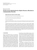
2.1 Illustration of the mapping between the solution space and the objective space. 8
2.2 Illustration of the (a) Pareto Dominance relationship between candidate so-
lutions relative to solution A and (b) the relationship between the Approxi-
mation Set, PF
A
and the true Pareto front, PF
∗
. 10
2.3 FrameworkofMOPSO 17
2.4 Illustration of pressure required to drive evolved solutions towards PF
∗
19
2.5 TrueParetofrontofKUR 29
2.6 TrueParetofrontofPOL 30
3.1 The process of archive updating . . . . . . . . . . . . . . . . . . . . . . . . . . 35
3.2 Searchregionoff-gbest 38
3.3 SPLS of assimilated particles along x1 and x3 . . . . . . . . . . . . . . . . . . 39
3.4 FlowchartofFMOPSO 40
3.5 Evolved tradeoffs by FMOPSO for a) ZDT1, b) ZDT4, c) ZDT6, d) FON, e)
KURandf)POL 42
3.6 Evolutionary trajectories in a) GD, b) MS, and c) S for ZDT1 . . . . . . . . . 42
3.7 Evolutionary trajectories in a) GD, b) MS, and c) S for ZDT4 . . . . . . . . . 43
3.8 Evolutionary trajectories in a) GD, b) MS, and c) S for ZDT6 . . . . . . . . . 43
3.9 Explored objective space FMOPSO at cycle a)20, b)40, c)60, d)80, e)100 and
SPLS only at cycle f)20, g)40, h)60, i)80, j)100 for ZDT1 . . . . . . . . . . . 43
3.10 Evolutionary trajectories in a) GD, b) MS, and c) S for ZDT1 . . . . . . . . . 44

3.11 Evolutionary trajectories in a) GD, b) MS, and c) S for ZDT4 . . . . . . . . . 45
3.12 Evolutionary trajectories in a) GD, b) MS, and c) S for ZDT6 . . . . . . . . . 45
3.13 Evolved tradeoffs by a) FMOPSO, b) CMOPSO, c) SMOPSO, d) IMOEA,
e) NSGA II, and f) SPEA2 for ZDT1 (PF
A
+ PF
∗
•) 50
vii
LIST OF FIGURES viii
3.14 Algorithm performance in a) GD, b) MS, and c) S for ZDT1 . . . . . . . . . 50
3.15 Evolutionary trajectories in a) GD, b) MS, and c) S for ZDT1 . . . . . . . . . 51
3.16 Evolved tradeoffs by a) FMOPSO, b) CMOPSO, c) SMOPSO, d) IMOEA,
e) NSGA II, and f) SPEA2 for ZDT4 (PF
A
× PF
∗
•) 52
3.17 Algorithm performance in a) GD, b) MS, and c) S for ZDT4 . . . . . . . . . 52
3.18 Evolutionary trajectories in a) GD, b) MS, and c) S for ZDT4 . . . . . . . . . 53
3.19 Evolved tradeoffs by a) FMOPSO, b) CMOPSO, c) SMOPSO, d) IMOEA,
e) NSGA II, and f) SPEA2 for ZDT6 (PF
A
× PF
∗
•) 54
3.20 Algorithm performance in a) GD, b) MS, and c) S for ZDT6 . . . . . . . . . 54
3.21 Evolutionary trajectories in a) GD, b) MS, and c) S for ZDT6 . . . . . . . . . 55
3.22 Evolved tradeoffs by a) FMOPSO, b) CMOPSO, c) SMOPSO, d) IMOEA,
e) NSGA II, and f) SPEA2 for FON (PF

A
× PF
∗
•) 55
3.23 Algorithm performance in a) GD, b) MS, and c) S for FON . . . . . . . . . . 56
3.24 Evolutionary trajectories in a) GD, b) MS, and c) S for FON . . . . . . . . . 56
3.25 Evolved tradeoffs by a) FMOPSO, b) CMOPSO, c) SMOPSO, d) IMOEA,
e) NSGA II, and f) SPEA2 for KUR (PF
A
+ PF
∗
•) 57
3.26 Algorithm performance in a) GD, b) MS, and c) S for KUR . . . . . . . . . . 57
3.27 Evolutionary trajectories in a) GD, b) MS, and c) S for KUR . . . . . . . . . 58
3.28 Evolved tradeoffs by a) FMOPSO, b) CMOPSO, c) SMOPSO, d) IMOEA,
e) NSGA II, and f) SPEA2 for POL (PF
A
+ PF
∗
•) 59
3.29 Algorithm performance in a) GD, b) MS, and c) S for POL . . . . . . . . . . 59
3.30 Evolutionary trajectories in a) GD, b) MS, and c) S for POL . . . . . . . . . 60
4.1 Framework of the competitive-cooperation model . . . . . . . . . . . . . . . . 68
4.2 Pseudocode for the adopted cooperative coevolutionary mechanism. . . . . . 71
4.3 Pseudocode for the adopted competitive co evolutionary mechanism. . . . . . 72
4.4 Flowchart of Competitive-Cooperative Co-evolutionary MOPSO . . . . . . . 74
4.5 Pareto fronts generated across 30 runs by (a) NSGAII, (b) SPEA2, (c) SIGMA,
(d) CCPSO, (e) IMOEA, (f) MOPSO, and (g) PAES for FON . . . . . . . . 77
4.6 Performance metrics of (a) GD, (b) MS, and (c) S for FON . . . . . . . . . . 77
4.7 Evolutionary trajectories in GD and N for FON . . . . . . . . . . . . . . . . . 78

4.8 Convergence behavior of CCPSO for FON . . . . . . . . . . . . . . . . . . . . 79
4.9 Performance metrics of (a) GD, (b) MS, and (c) S for KUR . . . . . . . . . . 79
LIST OF FIGURES ix
4.10 Evolutionary trajectories in GD and N for KUR . . . . . . . . . . . . . . . . 80
4.11 Convergence behavior of CCPSO for KUR . . . . . . . . . . . . . . . . . . . . 81
4.12 Pareto fronts generated across 30 runs by (a) NSGAII, (b) SPEA2, (c) SIGMA,
(d) CCPSO, (e) IMOEA, (f) MOPSO, and (g) PAES for ZDT4 . . . . . . . . 81
4.13 Performance metrics of (a) GD, (b) MS, and (c) S for ZDT4 . . . . . . . . . . 82
4.14 Evolutionary trajectories in GD, MS, S, and N for ZDT4 . . . . . . . . . . . 82
4.15 Pareto fronts generated across 30 runs by (a) NSGAII, (b) SPEA2, (c) SIGMA,
(d) CCPSO, (e) IMOEA, (f) MOPSO, and (g) PAES for ZDT6 . . . . . . . . 84
4.16 Performance metrics of (a) GD, (b) MS, and (c) S for ZDT6 . . . . . . . . . . 84
4.17 Evolutionary trajectories in GD, MS, S, and N for ZDT6 . . . . . . . . . . . 85
4.18 Box plots for GD by varying inertia weight . . . . . . . . . . . . . . . . . . . 86
4.19 Box plots for MS by varying inertia weight . . . . . . . . . . . . . . . . . . . 86
4.20 Box plots for S by varying inertia weight . . . . . . . . . . . . . . . . . . . . . 87
4.21 Box plots for GD by varying subswarm size . . . . . . . . . . . . . . . . . . . 88
4.22 Box plots for MS by varying subswarm size . . . . . . . . . . . . . . . . . . . 89
4.23 Box plots for S by varying subswarm size . . . . . . . . . . . . . . . . . . . . 89
4.24 Box plots for GD by varying archive size . . . . . . . . . . . . . . . . . . . . . 90
4.25 Box plots for MS by varying archive size . . . . . . . . . . . . . . . . . . . . . 91
4.26 Box plots for S by varying archive size . . . . . . . . . . . . . . . . . . . . . . 91
5.1 Pseudocode for the competitive coevolutionary mechanism in CPSO . . . . . 99
5.2 FlowchartofCPSO 100
5.3 TheModelofDCPSO 101
5.4 Schematic framework of DCPSO . . . . . . . . . . . . . . . . . . . . . . . . . 103
5.5 TheflowchartofDCPSO 104
5.6 Performance comparison of CPSO, CCEA and SPEA2 on a) GD, b) S, c)
MS,d)HVRforZDT1 108
5.7 Performance comparison of CPSO, CCEA and SPEA2 on a) GD, b) S, c)

MS,d)HVRforZDT2 109
5.8 Performance comparison of CPSO, CCEA and SPEA2 on a) GD, b) S, c)
MS,d)HVRforZDT3 110
5.9 Performance comparison of CPSO, CCEA and SPEA2 on a) GD, b) S, c)
MS,d)HVRforZDT4 111
LIST OF FIGURES x
5.10 Performance comparison of CPSO, CCEA and SPEA2 on a) GD, b) S, c)
MS,d)HVRforZDT6 112
5.11 Average runtime (in seconds) of DCPSO of five test problems and respective
no.ofpeers 114
5.12 Total average runtime of DCPSO with dynamic load balancing and without
dynamic load balancing for ZDT1 . . . . . . . . . . . . . . . . . . . . . . . . . 115
5.13 Total average runtime of DCPSO with dynamic load balancing and without
dynamic load balancing for ZDT2 . . . . . . . . . . . . . . . . . . . . . . . . . 115
5.14 Total average runtime of DCPSO with dynamic load balancing and without
dynamic load balancing for ZDT3 . . . . . . . . . . . . . . . . . . . . . . . . . 116
5.15 Total average runtime of DCPSO with dynamic load balancing and without
dynamic load balancing for ZDT4 . . . . . . . . . . . . . . . . . . . . . . . . . 116
5.16 Total average runtime of DCPSO with dynamic load balancing and without
dynamic load balancing for ZDT6 . . . . . . . . . . . . . . . . . . . . . . . . . 117
5.17 Performance comparison of DCPSO over different size of subswarms in GD
for a) ZDT1, b) ZDT2, c) ZDT3, d) ZDT4, e) ZDT6 . . . . . . . . . . . . . . 118
5.18 Performance comparison of DCPSO over different size of subswarms on Spac-
ing for a) ZDT1, b) ZDT2, c) ZDT3, d) ZDT4, e) ZDT6 . . . . . . . . . . . . 119
5.19 Performance comparison of DCPSO over different size of subswarms on Max-
imum Spread for a) ZDT1, b) ZDT2, c) ZDT3, d) ZDT4, e) ZDT6 . . . . . . 120
5.20 Performance comparison of DCPSO over different size of subswarms on Hy-
pervolumn Ratio for a) ZDT1, b) ZDT2, c) ZDT3, d) ZDT4, e) ZDT6 . . . . 121
6.1 Graphical representation of item and bin . . . . . . . . . . . . . . . . . . . . . 127
6.2 Flowchart of MOEPSO for solving the bin packing problem . . . . . . . . . . 130

6.3 The data structure of particle representation (10 item case) . . . . . . . . . . 131
6.4 Saving of bins with the inclusion of the orientation feature into the variable
lengthrepresentation 132
6.5 The insertion at new position when an intersection is detected at the top . . 134
6.6 The insertion at new position when an intersection is detected at the right . . 135
6.7 The insertion at next lower position with generation of three new insertion
points 135
6.8 Pseudo code for BLF heuristic . . . . . . . . . . . . . . . . . . . . . . . . . . 136
6.9 Pseudo code to check whether all rectangles can be inserted into the bin . . . 136
6.10 Initialization of initial solutions for the swarm of particles . . . . . . . . . . . 137
LIST OF FIGURES xi
6.11 Mechanism for updating position of particle . . . . . . . . . . . . . . . . . . . 139
6.12 Mutation modes for a single particle . . . . . . . . . . . . . . . . . . . . . . . 140
6.13 Partial swap of sequence between two bins in a particle . . . . . . . . . . . . 141
6.14 Intra bin shuffle within a bin of a particle . . . . . . . . . . . . . . . . . . . . 141
6.15 A sample input file of Class
3 1 11.txt 145
6.16 Evolution progress of the Pareto front . . . . . . . . . . . . . . . . . . . . . . 146
6.17 Two bins with the same deviation from idealized CG . . . . . . . . . . . . . . 147
6.18 Average deviation for different classes of items . . . . . . . . . . . . . . . . . 148
6.19 Pareto front to show the effectiveness of the PSO operator (Class
3 4 14) . . 149
6.20 Pareto front to show the effectiveness of the PSO operator (Class
4 10 10) . . 150
6.21 Pareto front to show the effectiveness of the mutation operator (Class
3 6 16) 151
6.22 Performance for Class
3 6 16: a) GD, b) MS and c) S . . . . . . . . . . . . . 151
6.23 Pareto front of Class
2 4 14 157

6.24 Performance for Class
2 4 14: a) GD, b) MS and c) S . . . . . . . . . . . . . 158
6.25 Evolutionary trajectories for Class
2 4 14: a) GD, b) MS and c) S . . . . . . 158
6.26 Pareto front of Class
3 4 14 159
6.27 Performance for Class
3 4 14: a) GD, b) MS and c) S . . . . . . . . . . . . . 159
6.28 Evolutionary trajectories for Class
3 4 14: a) GD, b) MS and c) S . . . . . . 160
6.29 Normalized computation time for the three algorithms . . . . . . . . . . . . . 161
List of Tables
2.1 Definition of ZDT test problems . . . . . . . . . . . . . . . . . . . . . . . . . 27
3.1 Performance of different features for ZDT1 . . . . . . . . . . . . . . . . . . . 46
3.2 Performance of different features for ZDT4 . . . . . . . . . . . . . . . . . . . 47
3.3 Performance of different features for ZDT6 . . . . . . . . . . . . . . . . . . . 48
3.4 Parameter settings of the different algorithms . . . . . . . . . . . . . . . . . . 49
3.5 Indices of the different algorithms . . . . . . . . . . . . . . . . . . . . . . . . . 49
4.1
Parameter setting for different algorithms 75
4.2 Indices of the different algorithms . . . . . . . . . . . . . . . . . . . . . . . . . 76
5.1 Parameter settings of the different algorithms . . . . . . . . . . . . . . . . . . 107
5.2 Specifications of the PC peers . . . . . . . . . . . . . . . . . . . . . . . . . . . 113
5.3 Configuration of the DCPSO simulation . . . . . . . . . . . . . . . . . . . . . 113
5.4 Average speedup of DCPSO for test problems and respective no. of peers . . 114
5.5 Total average runtime of DCPSO with dynamic load balancing and without
dynamic load balancing for ZDT1, ZDT2, ZDT3, ZDT4, and ZDT6 . . . . . . 117
6.1 Parameter settings used by MOEPSO in the simulation . . . . . . . . . . . . 143
6.2 Testcasesgeneration 144
6.3 Number of optimal solutions obtained by branch and bound method, EA,

PSOandEPSO(Class1-3) 155
6.4 Number of optimal solutions obtained by branch and bound method, EA,
PSOandEPSO(Class4-6) 156
6.5 Parameter settings used by MOEPSO in the simulation . . . . . . . . . . . . 157
xii
Chapter 1
Introduction
Optimization may be considered as a decision-making process to get the most out of available
resources for the best attainable results. Simple examples include everyday decisions, such
as what type of transport to take, which clothes to wear and what groceries to buy. For
these routine tasks, the decision to be made can be very simple. For example, most people
will choose the cheapest transport. Consider now, the situation where we are running
late for a meeting due to some unforseen circumstances. Since the need for expedition is
conflicting to the first consideration of minimizing cost, the selection of the right form of
transportation is no longer as straightforward as before and the final solution will represent
a compromise between the different objectives. This type of problems which involves the
simultaneous consideration of multiple objectives are commonly termed as multi-objective
(MO) problems.
Many real-world problems naturally involve the simultaneous optimization of several
competing objectives. Unfortunately, these problems are characterized by objectives that
are much more complex as compared to routine tasks mentioned above and the decision
space are often so large that it is often difficult, if not impossible, to be solved without
advanced and efficient optimization techniques. This thesis investigates the application of
an efficient optimization method, known as Particle Swarm Optimization (PSO), to the field
of MO optimization.
1
CHAPTER 1. 2
1.1 Motivation
Traditional operational research approaches to MO optimization typically entails the trans-
formation of the original problem into a SO problem and employs point-by-point algorithms

such as branch-and-bound to iteratively obtain a better solution. Such approaches have
several limitations including the generation of only one solution for each simulation run,
the requirement of the MO problem to be well-behaved, i.e. differentiability or satisfying
the Kuhn-Tucker conditions, and the sensitivity to the shape of the Pareto front. On the
other hand, metaheuristical approaches that are inspired by social, biological or physics phe-
nomena such as cultural algorithm (CA), particle swarm optimization (PSO), evolutionary
algorithm (EA), artificial immune system (AIS), differential evolution (DE), and simulated
annealing (SA) have been gaining increasing acceptance as much more flexible and effective
alternatives to complex optimization problems in the recent years. This is certainly a stark
contrast to just two decades ago, as Reeves remarked in [156] that an eminent person in
operational research circles suggested that using a heuristic was an admission of defeat!
MO optimization is a challenging research topic not only because it involves the si-
multaneous optimization of several complex objectives in the Pareto optimal sense, it also
requires researchers to address many issues that are unique to MO problems, such as fitness
assignment [45] [118], diversity preservation [96], balance between exploration and exploita-
tion [10], and elitism [108]. Many different CA, PSO, EA, AIS, DE and SA algorithms for
MO optimization have been proposed since the pioneering effort of Schaffer in [168], with
the aim of advancing research in above mentioned areas. All these algorithms are different in
methodology, particularly in the generation of new candidate solutions. Among these meta-
heuristics, multi-objective particle swarm optimization (MOPSO), which originates from the
simulation of behavior of bird flocks, is one of the most promising stochastic search method-
ology because of its easy implementation and high convergence speed. MOPSO algorithm
intelligently sieve through the large amount of information embedded within each particle
representing a candidate solution and exchange information to increase the overall quality
CHAPTER 1. 3
of the particles in the swarm.
This work seeks to explore and improve particle swarm optimization techniques for MO
function optimization as well as to expand its applications in real world bin packing prob-
lems. We will primarily use an experimental methodology backed up with statistical analysis
to achieve the objectives of this work. The effectiveness and efficiency of the proposed al-

gorithms are compared against other state of the art multi-objective algorithms using test
cases.
It is hoped that findings obtained by this study would give a better understanding of
PSO concept, and its advantages and disadvantages in application to MO problems. A
fuzzy up date strategy is designed to help PSO overcome difficulties in solving MO problems
with lots of local minimum. Coevolutionary PSO algorithm and distributed PSO algorithm
are implemented to reduce processing time in solving complex MO problems. And PSO is
also applied to bin packing problem to illustrate that PSO can be used to solve real world
combinatorial problems.
1.2 Contributions
1.2.1 MOPSO Algorithm Design
The design of fuzzy particle updating strategy and synchronous particle local search: The
fuzzy updating strategy models the uncertainty associated with the optimality of global best,
thus helping the algorithm to avoid undesirable premature convergence. The synchronous
particle local search performs directed local fine-tuning, which helps to discover a well-
distributed Pareto front. Experiment shows that balance between the exploration of fuzzy
update and the exploitation of SPLS is the key for PSO to solve complex MO problems.
Without them, PSO can not deal with multi-modal MO problems effectively.
The formation of a novel Competitive and Cooperative Coevolution Model for MOPSO:
As an instance of the divide-and-conquer paradigm, the proposed competitive and cooper-
CHAPTER 1. 4
ative coevolution model helps to produce reasonable problem decompositions by exploiting
any correlation or interdependency between subcomponents. This proposed method was val-
idated through comparisons with existing state of the art multiobjective algorithms through
the use of established benchmarks and metrics. The competitive and cooperative coevolu-
tion MOPSO is the only algorithm to attain the true Pareto front in all test problems, and
in all cases converges faster to the true Pareto front than any other algorithm used.
The implementation of Distributed Coevolutionary MOPSO: A distributed coevolution-
ary particle swarm optimization algorithm (DCPSO) is implemented to exploit the inherent
parallelism of coevolutionary particle swarm optimization. DCPSO is suitable for concur-

rent pro cessing that allows inter-communication of subpopulations residing in networked
computers, and hence expedites the computational speed by sharing the workload among
multiple computers.
1.2.2 Application of MOPSO to Bin Packing Problem
The mathematical formulation of two-objective, two-dimensional bin packing problems: The
bin packing problem is widely found in applications such as loading of tractor trailer trucks,
cargo airplanes and ships, where a balanced load provides better fuel efficiency and a safer
ride. In these applications, there are often conflicting criteria to be satisfied, i.e., to minimize
the bins used and to balance the load of each bin, subject to a number of practical con-
straints. Existing bin packing problem studies mostly focus on the minimization of wasted
space. And only Amiouny [3] has addressed the issue of balance (to make the center of grav-
ity of packed items as close as possible to target point). However Amiouny assumed that all
the items can be fitted into the bin, which will lead to bins with loosely packed items. In
this thesis, a two-objective, two-dimensional bin packing model (MOBPP-2D) is formulated
as no such model is available in literature. The minimum wasted space and the balancing
of load are the two objectives in MOBPP-2D, which provides a good representation for the
real-world bin packing problems.
CHAPTER 1. 5
The creative application of PSO concept on MOBPP-2D problem: The basic PSO con-
cept instead of the rigid original formula has been applied to solve multiobjective bin packing
problems. The best bin instead of the best solution is used to guide the search because bin
level permutation may keep more information about previous solutions and help avoid ran-
dom search. Multi-objective performance tests have shown that the proposed algorithm
performs consistently well for the test cases used.
In conclusion, although PSO is a relatively new optimization technique, our research
work has shown that PSO has great potential on solving MO problems. The successful
application to discrete bin packing problem also proves that PSO’s application is not limited
to continuous problem as it is originally designed.
1.3 Thesis Outline
This work is organized into seven chapters. The necessary concepts and definitions of multi-

objective optimization and particle swarm optimization algorithm are covered in Chapter 2.
It also presented an introduction to MOPSOs, with a general framework which illustrates
the basic design issues of the state-of-the-arts. Subsequently, a survey on the basic MO
algorithm components of fitness assignment, diversity maintenance and elitism is presented
to highlight the development trends of multi-objective problem solving techniques.
Chapter 3 addresses the issue of PSO’s fast convergence to local minimum. In par-
ticular, two mechanisms, fuzzy gbest and synchronous particle local search, are developed
to improve algorithmic performance. Subsequently, the proposed multi-objective particle
swarm optimization algorithm incorp orating these two mechanisms are validated against
existing multi-objective optimization algorithms.
Chapter 4 extends the notion of coevolution to decompose the problem and track the
optimal solutions in multi-objective particle swarm optimization. Most real-world multi-
objective problems are too complex for us to have a clear vision on how to decompose them
CHAPTER 1. 6
by hand. Thus, it is desirable to have a method to automatically decompose a complex
problem into a set of subproblems. This chapter introduces a new coevolutionary paradigm
that incorporates both competitive coevolution and cooperative coevolution observed in
nature to facilitate the emergence and adaptation of the problem decomposition.
Chapter 5 exploits the inherent parallelism of coevolutionary particle swarm optimiza-
tion to further formulate it into a distributed algorithm suitable for concurrent processing
that allows inter-communication of subp opulations residing in networked computers. The
proposed distributed coevolutionary particle swarm optimization algorithm expedites the
computational sp eed by sharing the workload among multiple computers.
Chapter 6 addresses the issue of solving bin packing problems using multi-objective par-
ticle swarm optimization. Analyzing the existing literature for solving bin packing problems
reveals that the current corpus has severe limitation as they focus only on minimization of
bins. In fact, some other important objectives, such as the issue of bin balance, also need
to be addressed for bin packing problems. Therefore, a multi-objective bin packing problem
is formulated and test problems are proposed. To accelerate the optimization process of
solving multi-objective bin packing problem, a multi-objective evolutionary particle swarm

optimization algorithm is implemented to explore the potential of high convergence speed
of PSO on solving multi-objective bin packing problem.
Chapter 7 gives the conclusion and directions for future work.
Chapter 2
Background Materials
2.1 MO Optimization
The specification of MO criteria captures more information about the real world problem as
more problem characteristics are directly taken into consideration. For instance, consider
the design of a system controller that can be found in process plants, automated vehicles
and household appliances. Apart from obvious tradeoff between cost and performance,
the performance criteria required by some applications such as fast response time, small
overshoot and good robustness, are also conflicting in nature and need to be considered
directly [21] [53] [114] [201].
Without any loss of generality, a minimization problem is considered in this work and
the MO problem can be formally defined as
min
x ∈

X
n
x

f(x )={f
1
(x),f
2
(x ), , f
M
(x)} (2.1)
s.t. g (x ) > 0,


h(x )=0
where x is the vector of decision variables bounded by the decision space

X
n
x
, and

f is the
set of objectives to be minimized. The terms “solution space” and “search space” are often
7
CHAPTER 2. 8
1
f
2
f
1
x
2
x
f
x
Solution space Objective space
Figure 2.1: Illustration of the mapping between the solution space and the objective space.
used to denote the decision space and will be used interchangeably throughout this work.
The functions g and

h represents the set of inequality and equality constraints that defines
the feasible region of the n

x
-dimensional continuous or discrete feasible solution space. The
relationship between the decision variables and the objectives are governed by the objective
function

f :

X
n
x
−→

F
M
. Figure 2.1 illustrates the mapping between the two spaces.
Depending on the actual objective function and constraints of the particular MO problem,
this mapping may not be unique.
2.1.1 Totally conflicting, nonconflicting, and partially conflicting MO prob-
lems
One of the key differences between SO (single objective) and MO optimization is that MO
problems constitute a multi-dimensional objective space

F
M
. This leads to three possi-
ble instances of MO problem, depending on whether the objectives are totally conflicting,
nonconflicting, or partially conflicting [193]. For MO problems of the first category, the
conflicting nature of the objectives are such that no improvements can be made without
violating any constraints. This result in an interesting situation where all feasible solutions
are also optimal. Therefore, totally conflicting MO problems are perhaps the simplest of the

CHAPTER 2. 9
three since no optimization is required. On the other extreme, a MO problem is nonconflict-
ing if the various objectives are correlated and the optimization of any arbitrary objective
leads to the subsequent improvement of the other objectives. This class of MO problem can
be treated as a SO problem by optimizing the problem along an arbitrarily selected objective
or by aggregating the different objectives into a scalar function. Intuitively, a single optimal
solution exist for such a MO problem.
More often than not, real world problems are instantiations of the third type of MO
problems with partially conflicting objectives and this is the class of MO problems that
we are interested in. One serious implication is that a set of solutions representing the
tradeoffs between the different objectives is now sought rather than an unique optimal
solution. Consider again the example of cost vs performance of a controller. Assuming
that the two objectives are indeed partially conflicting, this presents at least two possible
extreme solutions, one for lowest cost and one for highest performance. The other solutions,
if any, making up this optimal set of solutions represent the varying degree of optimality
with respect to these two objectives. Certainly, our conventional notion of optimality gets
thrown out of the window and a new definition of optimality is required for MO problems.
2.1.2 Pareto Dominance and Optimality
Unlike SO optimization where there is a complete order exist (i.e, f
1
≤ f
2
or f
1
≥ f
2
),

X
n

x
is partially-ordered when multiple objectives are involved. In fact, there are three possible
relationships among the solutions defined by Pareto dominance.
Definition 2.1: Weak Dominance:

f
1
∈

F
M
weakly dominates

f
2
∈

F
M
, denoted by

f
1


f
2
iff f
1,i
≤ f

2,i
∀i ∈{1, 2, ,M} and f
1,j
<f
2,j
∃j ∈{1, 2, , M}
Definition 2.2: Strong Dominance:

f
1
∈

F
M
strongly dominates

f
2
∈

F
M
, denoted by

f
1
≺

f
2

iff f
1,i
<f
2,i
∀i ∈{1, 2, , M}
Definition 2.3: Incomparable:

f
1
∈

F
M
is incomparable with

f
2
∈

F
M
, denoted by

f
1
∼

f
2
iff f

1,i
>f
2,i
∃i ∈{1, 2, , M} and f
1,j
<f
2,j
∃j ∈{1, 2, , M}
CHAPTER 2. 10
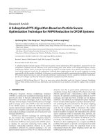
Figure 2.2: Illustration of the (a) Pareto Dominance relationship between candidate solu-
tions relative to solution A and (b) the relationship between the Approximation Set, PF
A
and the true Pareto front, PF
∗
.
With solution A as our point of reference, the regions highlighted in different shades of
grey in Figure 2.2(a) illustrates the three different dominance relations. Solutions located
in the dark grey regions are dominated by solution A because A is better in both objectives.
For the same reason, solutions located in the white region dominates solution A. Although
A has a smaller objective value as compared to the solutions located at the boundaries
between the dark and light grey regions, it only weakly dominates these solutions by virtue
of the fact that they share a similar objective value along either one dimension. Solutions
located in the light grey regions are incomparable to solution A because it is not possible
to establish any superiority of one solution over the other: solutions in the left light grey
region are better only in the second objective while solutions in the right light grey region
are better only in the first objective.
With the definition of Pareto dominance, we are now in the position to consider the set
of solutions desirable for MO optimization.
Definition 2.4: Pareto Optimal Set (PS
∗

): The Pareto optimal set is the set of nondomi-
nated solutions such that PS
∗
= {x
∗
i
|

F (x
j
) ≺

F (x
∗
i
),

F(x
j
) ∈

F
M
}.
CHAPTER 2. 11
Definition 2.5: Pareto Optimal Front (PF
∗
): The Pareto optimal front is the set of objec-
tive vectors of nondominated solutions such that PF
∗

= {

f
∗
i
|

f
j
≺

f
∗
i
,

f
j
∈

F
M
}.
The nondominated solutions are also termed “noninferior”, “admissible” or “efficient” so-
lutions. Each objective component of any nondominated solution in the Pareto optimal set
can only be improved by degrading at least one of its other objective components [184].
2.1.3 MO Optimization Goals
An example of the PF
∗
is illustrated in Figure 2.2(b). Most often, information regarding the

PF
∗
are either limited or not known a priori. It is also not easy to find a nice closed analytic
expression for the tradeoff surface because real-world MO problems usually have complex
objective functions and constraints. Therefore, in the absence of any clear preference on the
part of the decision-maker, the ultimate goal of multi-objective optimization is to discover
the entire Pareto front. However, by definition, this set of objective vectors is possibly an
infinite set as in the case of numerical optimization and it is simply not achievable.
On a more practical note, the presence of too many alternatives could very well over-
whelm the decision-making capabilities of the decision-maker. In this light, it would be more
practical to settle for the discovery of as many nondominated solutions possible as compu-
tational resources permits. More precisely, the goal is to find a good approximation of the
PF
∗
and this approximate set, PF
A
should satisfy the following optimization objectives.
• Minimize the distance between the PF
A
and PF
∗
.
• Obtain a good distribution of generated solutions along the PF
A
.
• Maximize the spread of the discovered solutions.
An example of such an approximation is illustrated by the set of nondominated solu-
tions denoted by the filled circles residing along the PF
∗
in Figure 2.2(b). While the first

optimization goal of convergence is the first and foremost consideration of all optimization
CHAPTER 2. 12
problems, the second and third optimization goal of maximizing diversity are unique to MO
optimization. The rationale of finding a diverse and uniformly distributed PF
A
is to pro-
vide the decision maker with sufficient information about the tradeoffs among the different
solutions before the final decision is made. It should also be noted that the optimization
goals of convergence and diversity are somewhat conflicting in nature, which explains why
MO optimization is much more difficult than SO optimization.
2.2 Particle Swarm Optimization Principle
Particle swarm optimization (PSO) was first introduced by James Kennedy (a social psy-
chologist) and Russell Eb erhart (an electrical engineer) in 1995 [92], which originates from
the simulation of behavior of bird flocks. Although a number of scientists have created com-
puter simulations of various interpretations of the movement of organisms in a bird flock or
fish school, Kennedy and Eberhart became particularly interested in the models developed
by Heppner (a zoologist) [62].
In Heppner’s model, birds would begin by flying around with no particular destination
and in spontaneously formed flo cks until one of the birds flew over the roosting area. To
Eberhart and Kennedy, finding a roost is analogous to finding a good solution in the field of
possible solutions. And they revised Heppner’s methodology so that particles will fly over
a solution space and try to find the best solution dep ending on their own discoveries and
past experiences of their neighbors.
In the original version of PSO, each individual is treated as a volume-less particle in
the D dimensional solution space. The equations for calculating velocity and position of
particles are shown below:
v
k+1
id
= v

k
id
+ r
k
1
× p × sgn(p
k
id
− x
k
id
)+r
k
2
× g × sgn(p
k
gd
− x
k
id
) (2.2)
x
k+1
id
= x
k
id
+ v
k
id

(2.3)