Development of higher order triangular element for accurate stress resultants in plated and shell structures 6

CHAPTER 5

222




Nonlinear Continuum
Spectral Shell Element



In Chapter
4
, we presented a detailed derivation of HT-CS and HT-CS-X
elements, the associated linear
finite element formulation and several
challenging benchmark problems to assess the performances of higher order
elements. Based on the performances of HT-CS and HT-CS-X elements in
‘Discriminating and Revealing Test Cases’, it was found that HT-CS-X

elements are more robust in handling a wide range of shell problems. Further,
the element was also tested for its capability to handle stress resultants in
challenging linear plate bending problems (Morley’s skew plate and corner
supported square plate). Having assessed the performance of HT-CS-X
element in linear plate\shell analysis, in this chapter, we shall extend the linear
finite element formulation of HT-CS-X elements to a nonlinear formulation
that caters for large deflection problems. The performance of the developed
nonlinear continuum shell element will be assessed in several geometric
nonlinear shell
problems
. Moreover, its superiority over lower order elements
in handling
stresses in the nonlinear regime

will be discussed
.


The large deflection analysis of shells has drawn the attention of many
researchers due to its importance in engineering practice. There have been
numerous research studies on the geometric nonlinear analysis of shells that
undergo large deflections, moderate\finite rotations (see for example, Simo et






Nonlinear Continuum Spectral Shell Element

223
al.,1989; Saleeb et al, 1990; Sze et al., 1999; Balah and Al-Ghamedy, 2002;
Arciniega and Reddy,
2007). Most of the researchers presented
the nonlinear
load versus deflection response of shell structures computed from various
kinds of
shell elements that were developed to tackle nonlinear behaviour. The
ability of finite elements
in handling stresses in nonlinear regime has received
relatively less attention. The accurate prediction of stress distributions in the
nonlinear region is very crucial from a design point of view. Furthermore, the
correct estimation of peak stresses and their localization in nonlinear region
provides a sound basis to perform reliability and failure studies which decide
the safety of a structural component. Achieving good and reliable levels of
accuracy in the highly nonlinear range with lesser computational resources is
certainly not possible with lower order finite elements. Although the nonlinear
load versus deflection response of the structure may be traced accurately with
coarser mesh designs of lower order finite elements, one may require very fine
mesh designs in order to achieve good accuracy of stress values. Furthermore,
the accuracy of stresses predicted by lower order elements may be highly
erroneous in problems which involve steep stress gradients. Hence, we use
higher order finite elements that
have enriched shape functions and render
many advantages over conventional lower order finite elements such as the
accommodation of high aspect ratio elements, better prediction of stresses
with coarser meshes, ability to handle steep stress gradients, less sensitivity to
input data (locking mechanisms) and lesser computational resources as
compared to lower order finite elements.

In this chapter,
we shall present
the nonlinear finite element formulation of
a continuum shell element that accounts for
large deflections and moderate






Nonlinear Continuum Spectral Shell Element

224
rotations of shell structures. The accuracy of the proposed element will be
verified via
several n
onlinear benchmark problems and their superior
performance over conventional lower order shell finite elements will be
illustrated in
the

nonlinear stress analysis

of
the shell problems.


This chapter has been organized into four

main sections.
The first section
deals with the development of nonlinear finite element model for shells under
the framework of Total Lagrangian approach followed by a description on
nonlinear solution algorithms adopted in the present work. In the second
section, we verify the performance of HT-CS-X elements in selected nonlinear
shell benchmark problems. Following this, we will present the performance of
HT-CS-X elements in handling stresses in nonlinear region much efficiently as
compared to ABAQUS S8R lower order shell elements. The performances of
HT-CS-X element and ABAQUS S8R element will be compared in the
context of accuracy and distribution of stresses, relative ease of mesh designs
and number of degrees of freedom to achieve a smooth stress variation. In the
last section of this chapter, we will present a
detailed nonlinear analysis of
laminated composite hyperboloid shells
which are challen
ging due to their
negative value of Gaussian curvature and complex behaviour.


5.1 Description of motion
Consider a deformable body of known geometry, constitution and loading that
occupies
an initial
configuration Â
0

in which a particle X occupies the position
X
having Cartesian coordinates (

X, Y, Z). After the application of loads, the
body assumes a new position x
in the deformed configuration
Â
having
coordinates (x, y, z). The objective is to determine the final configuration of a
body subjected to a total load say P
max
. A straightforward way of determining






Nonlinear Continuum Spectral Shell Element

225
the final configuration Â
from a known initial configuration
Â
0

is to assume
that the total load P
max
is applied in increments so that the body occupies
several intermediate configurations Â
i
(i =1,2,……) prior to attaining the final

configuration. The magnitude of load increments should be such that the
computational procedure that is employed to trace the response of the body
(such as the Newton Raphson method and the
Arc
-length method) is capable
of predicting the deformed configuration at the end of each load step. In the
determination of an intermediate configuration Â
i
, one may use any of the
previously known configurations Â
0
, Â
1
, … ,Â
i-1
as the reference
configuration Â
R
. If the initial configuration is used as the reference
configuration with respect to which all quantities are measured, it is called the
Total Lagrangian description.


We consider three equilibrium configurations of the body namely, Â
0
, Â
1
and Â
2

which correspond to three dif
ferent loads. Â
0
denotes the initial
undeformed configuration, Â
1
denotes the last known deformed configuration
and Â
2
denotes the current deformed configuration to be determined. It is
assumed that all variables such as displacements, strains and stresses
are
known up to configuration Â
1
. The objective is to develop a formulation
to
determine the displacements and stresses of the body in the deformed
configuration Â
2
.

In the nex
t section, we present the strain and stress measures employed in
the Total Lagrangian formulation. A detailed derivation of relevant stress and
strain measures for a Total Lagrangian approach can be seen in standard
textbooks on nonlinear finite element formulation
(Reddy
, 2004). Hence we

Nonlinear Continuum Spectral Shell Element

226
present the final equations that are necessary for the development of nonlinear
finite element model.
5.1.1 Green strain tensor
We adopt the Green-Lagrange strain tensor or simply referred to as the Green
strain tensor to measure the deformation of a body. The Green strain tensor is
symmetric and is expressed as follows:


( )
( )
ICIFFE
T
-=-ì=
2
1
2
1

(5.1)

where
FFC
T

ì=
is called the right Cauchy-Green deformation tensor
and
F

is the deformation gradient tensor defined as


=
ữ
ứ
ử
ỗ
ố
ổ
ả
ả
=
T
X
x
F


ỳ
ỳ
ỳ
ỳ
ỳ
ỳ

ỳ
ỷ
ự
ờ
ờ
ờ
ờ
ờ
ờ
ờ
ở
ộ
ả
ả
ả
ả
ả
ả
ả
ả
ả
ả
ả
ả
ả
ả
ả
ả
ả
ả

z
z
y
z
x
z
z
y
y
y
x
y
z
x
y
x
x
x
0
1
0
1
0
1
0
1
0
1
0
1

0
1
0
1
0
1








(5.2)


The Green strain tensor can be written as


ữ
ữ
ứ
ử
ỗ
ỗ
ố
ổ
ả
ả

ả
ả
+
ả
ả
+
ả
ả
=
J
K
I
K
I
J
J
I
JI
X
u
X
u
X
u
X
u
E
2
1

(5.3)
where
I
u
denotes the component of displacement. The subscripts I,J,K
take
the values
of

1,2,3 (
uu =
1
,
vu =
2

and
wu =
3
). u, v
denote the in
-plane
displacements and w denotes the transverse displacements. Likewise,

I
X

denotes the components of Cartesian coordinates (
XX =
1
,
YX =
2

and
ZX =
3
).










Nonlinear Continuum Spectral Shell Element

227
The Green-strain components can be written as

ỳ
ỳ
ỷ
ự
ờ
ờ
ở
ộ
ữ
ứ
ử
ỗ
ố
ổ
ả
ả
+
ữ
ứ
ử
ỗ
ố
ổ
ả
ả
+
ữ
ứ

ử
ỗ
ố
ổ
ả
ả
+
ả
ả
=
222
2
1
X
w
X
v
X
u
X
u
E
xx



ỳ
ỳ
ỷ
ự

ờ
ờ
ở
ộ
ữ
ứ
ử
ỗ
ố
ổ
ả
ả
+
ữ
ứ
ử
ỗ
ố
ổ
ả
ả
+
ữ
ứ
ử
ỗ
ố
ổ
ả
ả

+
ả
ả
=
222
2
1
Y
w
Y
v
Y
u
Y
v
E
yy



ỳ
ỳ
ỷ
ự
ờ
ờ
ở
ộ
ữ
ứ

ử
ỗ
ố
ổ
ả
ả
+
ữ
ứ
ử
ỗ
ố
ổ
ả
ả
+
ữ
ứ
ử
ỗ
ố
ổ
ả
ả
+
ả
ả
=
222
2

1
Z
w
Z
v
Z
u
Z
w
E
zz



ữ
ứ
ử
ỗ
ố
ổ
ả
ả
ả
ả
+
ả
ả
ả
ả
+

ả
ả
ả
ả
+
ả
ả
+
ả
ả
=
Y
w
X
w
Y
v
X
v
Y
u
X
u
X
v
Y
u
E
yx
2

1



ữ
ứ
ử
ỗ
ố
ổ
ả
ả
ả
ả
+
ả
ả
ả
ả
+
ả
ả
ả
ả
+
ả
ả
+
ả
ả

=
Z
w
X
w
Z
v
X
v
Z
u
X
u
X
w
Z
u
E
zx
2
1



ữ
ứ
ử
ỗ
ố
ổ

ả
ả
ả
ả
+
ả
ả
ả
ả
+
ả
ả
ả
ả
+
ả
ả
+
ả
ả
=
Z
w
Y
w
Z
v
Y
v
Z

u
Y
u
Y
w
Z
v
E
zy
2
1




(5.4)
5.1.2 Stress tensor
The equation of equilibrium has
to be derived for the deformed configuration
of the body,
i.e
.
at configuration

2
. Since the geometry of the deformed
configuration is unknown, the equations are written in terms of the known
reference configuration
0
. In doing so, it becomes necessary to introduce

various measures of stress. These stress measures emerge when the elemental
volumes and areas are transformed from the deformed configuration to the
undeformed configuration. In the Total Lagrangian approach we use the
second Piola-Kirchhoff stress tensor denoted as S. The second Piola-Kirchhoff
stress S
can be expressed in terms of Cauchy stress tensor
s

(which is defined
to be the current force per unit deformed area) by the following transformation




T
FJFS

ìì= s
1




(5.5)

Nonlinear Continuum Spectral Shell Element

228
where,
J

denotes the determinant of the deformation gradient tensor
F
. The
second Piola-Kirchhoff stress tensor S, gives the transformed current force per
unit undeformed area. The stress tensor S
is symmetric whenever the Cauchy
stress tensor s
is symmetric.
For details on the transformation of various
measures one may refer to books by Bathe (1996) and Reddy (2004).


Having mentioned about the strain and stress measures, it can be shown
that the rate of internal work done in a continuous medium in the current
configuration can be expressed as
(
Reddy 2004):




dVESW
V
ò

=
&
:
2
1




(5.6)
Thus the second Piola-Kirchhoff tensor S is the work conjugate to the rate of
the Green-Lagrange strain tensor
E
&
. The following notations are used in this
chapter. A left superscript on a quantity denotes the configuration in which the
quantity occurs and a left subscript denotes the configuration with respect to
which the quantity is measured. For example,
H
i
j
refers to a quantity H
(say
displacements, stresses) that occurs in configuration Â
i

but is measured in
configuration Â
j
. When the quantity is measured in the same configuration,

the left subscript is omitted. The left superscript will be omitted for all
incremental quantities that occur between configurations Â
1
and Â
2
. The right
subscript refers to the components of Cartesian coordinate system.


When the body deforms under the action of externally applied loads, a
particle X occupying position (X, Y, Z) in configuration Â
0
moves to a new
position x
having coordinates
(x, y, z) in configuration Â
2
. The components of
particle X can be written as
( )
zyxx
0000
,,=

and that of
x can be written

Nonlinear Continuum Spectral Shell Element

229
as
( )
zyxx
2222
,,=
. The total displacements of a particle X
in the two
configurations Â
1
and Â
2
can be written as:








iii
xxu
011
0
-=

,
(i
=1,2,3)



(5.7 a)








iii
xxu
022
0
-=
,
(
i
=1,2,3)

(5.7 b)
The displacement increment of a point from configuration Â
1

to
Â
2
is






iii
uuu
1
0
2
0
-=
, (i
=1,2,3)

(5.8)
5.1.3 Green Strain tensor and
stress tensor
for various
configurations

The components of Green strain tensor in configurations Â
1
and Â
2

are given

in terms of displacements as:


÷
÷
ø
ö
ç
ç
è
æ
¶
¶
¶
¶
+
¶

¶
+
¶
¶
=
j
k
i
k
i
j
j
i
ij
x
u
x
u
x
u
x
u
E
0
1
0
0
1
0
0

1
0
0
1
0
1
0
2
1






(5.9 a)


÷
÷
ø
ö
ç
ç
è
æ
¶
¶
¶
¶

+
¶
¶
+
¶
¶
=
j
k
i
k
i
j
j
i
ij
x
u
x
u
x
u
x
u
E
0
2
0
0
2

0
0
2
0
0
2
0
2
0
2
1






(5.9 b)
The incremental Green-Lagrange strain components
ij
e
0
which are obtained
in moving from configuration Â
1
to Â
2
are given as

jijiji
e he
000
+=








(5.10)
where,
ji
e
0

are linear components of strain increm
ent tensor expressed as




÷
÷
ø
ö
ç
ç

è
æ
¶
¶
¶
¶
+
¶
¶
¶
¶
+
¶
¶
+
¶
¶
=
j
k
i
k
j
k
i
k
i
j
j
i

ji
x
u
x
u
x
u
x
u
x
u
x
u
e
0
1
0
000
1
0
00
0
2
1


(5.11)
The nonlinear components
ji
h

0

are given by





j
k
i
k
ji
x
u
x
u
00
0
2
1
¶
¶
¶
¶
=h

(5.12)






Nonlinear Continuum Spectral Shell Element

230
For geometrically linear analysis, only two configurations Â
1
= Â
0

and
Â
2

are
involved.
Thus
0
1
=
i
u
and
ii
uu =

2
. The terms involving products of
( )
ik
xu
0
¶¶

and
( )
jk
xu
0
¶¶

are small and hence are neglected. Consequently,
the linear components of strain increment tensor
ji
e
0
become the same as the
components of the Green-Lagrange strain tensor
ij
E
2
0

and both reduce to
infinitesimal strain components

÷
÷
ø
ö
ç
ç
è
æ
¶
¶
+
¶
¶
=
i
j
j
i
ji
x
u
x
u
e
00
0
2
1

(5.13)
The second Piola-Kirchhoff stress tensor components in configurations Â
1

and
Â
2

are denoted by
ji
S
1
0

and
ji
S
2
0

respectively. They are re
lated by the
following equation

jijiji
SSS
0
1
0
2
0
+=




(5.14)
where,
ji
S
0

are the components of the Kirchhoff

stress increment tensor and
are given by:


lkijklji
CS e
000
=

(5.15)
ijkl
C
0

denotes the in
cremental constitutive tensor with respect to configuration
Â
0
. In the present work, since we deal with geometric nonlinearity, the
components of the constitutive matrix are the same as that obtained for a linear
analysis.
5.1.4 Total Lagrangian Formulation
Having defined the necessary terms involved in the Total Lagrangian
formulation, we now present the final equations of equilibrium. The equations
of Lagrangian incremental description of motion for the displacement based






Nonlinear Continuum Spectral Shell Element

231
finite element model considered herein are derived from the principle of
virtual displacements. The detailed derivation of the equations of equilibrium
can be found in

the book by
Reddy (2004).


The weak form of the equilibrium equation that is suited for the
development of displacement finite element model based on the Total
Lagrangian formulation is given to be:


òò
-=+
V
jiji
V
jilklkji
RRVdSVdeeC
00
)()()()(
1
0
2
0
0
0
1
0
0
000
ddhdd

(5.16)
where
( )
( )
VdeSR
V
jiji
0
0
1
0
1
0
0
ò
= dd
is the equivalent nodal force vector
and
( )
SdutVdufR
S
ii
V
ii
02
0
02
0
2

0
00
òò
+= ddd
is the externally applied load vector
(sum of body force and traction force). The total stress components
ji
S
1
0

are
evaluated using the following constitutive relation


lklkjiji
ECS
1
00
1
0
=




(5.17)
where,
lk
E

1
0

are the Green
-Lagrange strain components described in Eq. (5.4).
5.2 Finite Element Model Continuum
Shell Element

The equilibrium equation that is required for the development of nonlinear
displacement based degenerated shell finite element model for a solid
continuum is given in Eq. (5.16). In order to derive the finite element
equations for a shell element, the first step is to select appropriate interpolation
(shape) functions for the displacement field and geometry. The coordinates
and displacements are interpolated using the isoparametric concept which
involves the same interpolation functions. This is done to ensure the
displacement compatibility across element boundaries is preserved at all
configurations






Nonlinear Continuum Spectral Shell Element

232


The degenerated
shell element is deduced from the 3D continuum element

by imposing two kinematic constraints, i.e. (i) the straight line normals to the
midsurface before deformation remain straight but not necessarily normal after
deformation, allowing for the effect of transverse shear deformation and (ii)
transverse normal strain/stress components are neglected, allowing for the
conversion of the 3D shell model into a 2D model. Moreover, the strains are
assumed to be small.


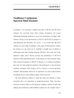
The layout of HT-CS-X is shown in Fig. 5.1 with Lobatto nodal
distribution in the element. In Fig. 5.1, r
and
s denote the curvilinear
coordinates of the element and t denotes the coordinate in the thickness
direction.

The global Cartesian coordinates (
x, y, z) of a point on the element are
defined as follows:





( )
ỳ
ỳ
ỳ
ỷ
ự
ờ

ờ
ờ
ở
ộ
ù
ỵ
ù
ý
ỹ
ù
ợ
ù
ớ
ỡ
ữ
ứ
ử
ỗ
ố
ổ
-
+
ù
ỵ
ù
ý
ỹ
ù
ợ
ù

ớ
ỡ
ữ
ứ
ử
ỗ
ố
ổ
+
Q=
ù
ỵ
ù
ý
ỹ
ù
ợ
ù
ớ
ỡ
ồ
=
bottom
i
i
i
top
i
i
i

i
i
z
y
x
t
z
y
x
t
sr
z
y
x
2
1
2
1
,
45
1


(5.18)


Fig. 5.1 Layout of HT-CS-X element having optimally located Lobatto nodes

Nonlinear Continuum Spectral Shell Element

233
ii
yx ,

and
i
z
denote
the coordinates in

the
x, y
and
z direction at node i. In Fig.
5.1,
1
ˆ
E
,
2
ˆ
E

and

3
ˆ
E

denote the unit vectors defined along the global (
x, y, z)
coordinate system. Let
i
V
3

be a vector connecting

the upper and lower points
of the shell’s normal at node i, i.e.




bottom
i
i
i
top
i
i
i
i
z
y

x
z
y
x
V
ï
þ
ï
ý
ü
ï
î
ï
í
ì
-
ï
þ
ï
ý
ü
ï
î
ï
í
ì
=
3

(5.19)
The corresponding unit vector is defined as
iii
VVe
333
ˆ
=
. Equation (5.18) can
now be written as

( ) ( )
ú
ú
ú
û
ù
ê
ê
ê
ë
é
+
ï
þ
ï
ý
ü
ï

î
ï
í
ì
Q=
ú
ú
ú
û
ù
ê
ê
ê
ë
é
+
ï
þ
ï
ý
ü
ï
î
ï
í
ì
Q=
ï
þ
ï

ý
ü
ï
î
ï
í
ì
åå
==
i
i
midsurface
i
i
i
i
i
i
midsurface
i
i
i
i
i
eh
t
z
y
x
srV

t
z
y
x
sr
z
y
x
3
45
1
3
45
1
2
,
2
,


(5.20)
where
i
i
Vhh
3
==

is the thickness of the shell at node
i. The curvature of the

shell is described in terms of the shell director vector
i
V
3
. When the director
vector has no components in the x
and
y
directions, the corresponding unit
vector
i
e
3
ˆ

becomes a unit vector in the global
z
direction and the resulting
structure represents a plate.
The displacements and incremental displacements are given by:


ú
û
ù
ê
ë
é
-+Q=-=
å

=
)(
2
),(
3
0
3
11
45
1
1
011 k
i
k
ik
k
i
k
kii
eeh
t
usrxxu




(5.21)

ú
û
ù
ê
ë
é
-+Q=-=
å
=
)(
2
),(
3
1
3
2
45
1
12 k
i
k
ik
k
i
k
kiii
eeh
t
usruuu

(5.22)







Nonlinear Continuum Spectral Shell Element

234
Here
k
i
u
1

and
k
i
u
denote, respectively, the displacement and incremental
displacement components in
i
x
direction at the

k
th

node.

By substituting Eqs.
(5.20),
(
5.21)
and
(5.22) into Eq. (5.16), the finite element model is given by


{ }
}{}]){[][(
1
0
2
1
0
1
0
FRKK
e
NLL
-=+ D

(5.23)
where,
}{
e
D
is the vector of nodal incremental displacements from time t to
time t
+
D
t in an element, and
][
1
0 L
K
}{
e
D
,
][
1
0 NL
K
}{
e
D

and
}{
1
0

F

are obtained
by evaluating the following integrals






VdBCBK
L
V
T
LL
01
00
1
0
1
0
][][][][
0
ò
=


(5.24a)

VdBSBK
NL
V
T
NLNL
01
0
1
0
1
0
1
0
][][][][
0
ò
=


(5.24b)




VdSBF
V
T
L

01
0
1
0
1
0
}
ˆ
{][}{
0
ò
=




(5.24c)
in which
][
1
0 L
B

and
][
1
0 NL
B

are the linear and nonlinear strain

–displacement
transformation matrices,
][
0
C

is the incremental stress
-strain material property
matrix,
][
1
0
S

is a matrix of 2
nd

Piola
-Kirchhoff stress components,
}
ˆ
{
1
0
S
is a
vector of these stresses and
{ }
R
2

is the vector of applied loads. All matrix
elements are defined with respect to the
configuration
Â
0

and the solution at
Â
2

is sought. Equation (
5.23) represents the nonlinear equilibrium equation
and has to be iterated for each time step until it satisfies a specified tolerance
in the displacements.
When the shell director undergoes small rotation
Wd

at each node we have



kkkkkk
eeed
3
1
32
1
11
1

2
ˆˆˆ
qqq ++=W




(5.25)
The increment of vector
k
e
3
1
ˆ

can be written as



kkkkkkkk
eeedeee
2
1
21
1
13
1
3
1
3

2
3
1
ˆˆˆˆˆˆ
qq -=´W=-=D


(5.26)






Nonlinear Continuum Spectral Shell Element

235
Hence, Eq. (5.22) can be expressed as


)3,2,1()
ˆˆ
(
2
),(
2
1
21
1
1

45
1
=
ú
û
ù
ê
ë
é
-+Q=
å
=
ieeh
t
usru
k
i
kk
i
k
k
k
i
k
ki
qq

(5.27)
The unit vectors
k
e
1
1
ˆ

and
k
e
2
1
ˆ

at node
k
can be obtained from the relations





kkk
k
k
k
eee
eE
eE

e
1
1
3
1
2
1
3
1
2
3
1
2
1
1
ˆˆˆ
,
ˆ
ˆ
ˆ
ˆ
ˆ
´=
´
´
=

(5.28)
where
i
E
ˆ
are the unit vectors of the stationary global Cartesian coordinate
system
),,(
000
zyx
.
The incremental displacement vector can be written in matrix form as


{ } { }
[ ]
( )
{ }
( )
1455
4553
1
321
´´
´´
D==
e
T

Huuuu


(5.29)
where
{ } { }
T
kkk
i
e
u
21
qq=D
,(i = 1, 2, 3, k
= 1, 2,…,
45) is the vector of nodal
incremental displacements (five per node).
[ ]
H
1

is the incremental
displacement interpolation matrix
given by

[ ]
( )
ú
ú
ú

ú
ú
ú
û
ù
ê
ê
ê
ê
ê
ê
ë
é
Q-QQ
Q-QQ
Q-QQ
=
´´
KK
KK
KK
k
kk
k
kkk
k
kk
k
kkk
k

kk
k
kkk
ehteht
ehteht
ehteht
H
23
1
13
1
22
1
12
1
21
1
11
1
4553
1
2
1
2
1
00
2
1
2
1

00
2
1
2
1
00


(5.30)
The linear strain increments
{ }
T
zyzxyxzzyyxx
eeeeeee }222{
0000000
=

are expressed in matrix form as


{ }
}{][
0
1
0
uAe =

(5.31)
where,
{ }
T
z
w
y
w
x
w
z
v
y
v
x
v
z
u
y
u
x
u
u
¶

¶
¶
¶
¶
¶
¶
¶
¶
¶
¶
¶
¶
¶
¶
¶
¶
¶
=
000000000
0
are
the vector derivatives of increment displacements.






Nonlinear Continuum Spectral Shell Element

236
[ ]
ú
ú
ú
ú
ú
ú
ú
ú
ú
ú
ú
ú
ú
ú
ú
ú
û
ù
ê
ê
ê
ê
ê
ê
ê
ê
ê
ê

ê
ê
ê
ê
ê
ê
ë
é
¶
¶
¶
¶
+
¶
¶
+
¶
¶
¶
¶
¶
¶
¶
¶
¶
¶
+
¶
¶
¶

¶
¶
¶
+
¶
¶
¶
¶
¶
¶
¶
¶
¶
¶
+
¶
¶
+
¶
¶
¶
¶
+
¶
¶
¶
¶
¶
¶
¶

¶
+
¶
¶
¶
¶
¶
¶
¶
¶
+
=
´
y
w
z
w
y
v
z
v
y
u
z
u
x
w
z
w
x

v
z
v
x
u
z
u
x
w
y
w
x
v
y
v
x
u
y
u
z
w
z
v
z
u
y
w
y
v
y

u
x
w
x
v
x
u
A
1
0
1
0
1
0
1
0
1
0
1
0
1
0
1
0
1
0
1
0
1
0

1
0
1
0
1
0
1
0
1
0
1
0
1
0
1
0
1
0
1
0
1
0
1
0
1
0
1
0
1
0

1
0
96
1
10100
01010
00101
1000000
0001000
0000001








(5.32)
The vectors
{ }
u
0

and
{ }
e
0

are related to the displacement increments at nodes

by the following equations.


{ }
[ ]
{ }
[ ] [ ]
{ }
e
Huu DP=P=
1
0




(5.34)


{ }
[ ]
{ }
[ ][ ] [ ]
{ }
[ ]
{ }
ee
BHAuAe D=DP==
1
0

11
0
1
0


(5.35)




[ ] [ ][ ] [ ]
HAB
111
0
P=






(5.36)
where,
[ ]
T
P
is the operator of differentials
given by

[ ]
ú
ú
ú
ú
ú
ú
ú
û
ù
ê
ê
ê
ê
ê
ê
ê
ë
é
¶
¶
¶
¶
¶
¶
¶
¶
¶
¶
¶

¶
¶
¶
¶
¶
¶
¶
=P
zyx
zyx
zyx
T
000
000
000
000000
000000
000000




(5.37)
The components of
][
1
A

include

the

derivatives of displacements denoted by

ji
u
,
1
0

( )
.
0
,0 jiji
xuu ¶¶=
Hence the derivatives of these displacements
ji
u
,
1
0
with respect to the global coordinates
x
0
,
y
0
and
z
0

are obtained through
the relation






Nonlinear Continuum Spectral Shell Element

237
[ ]
ú
ú
ú
ú
ú
ú
ú
û
ù
ê
ê
ê
ê
ê
ê
ê
ë
é

¶
¶
¶
¶
¶
¶
¶
¶
¶
¶
¶
¶
¶
¶
¶
¶
¶
¶
=
ú
ú
ú
ú
ú
ú
ú
û
ù
ê
ê

ê
ê
ê
ê
ê
ë
é
¶
¶
¶
¶
¶
¶
¶
¶
¶
¶
¶
¶
¶
¶
¶
¶
¶
¶
=
-
t
w
t

v
t
u
s
w
s
v
s
u
r
w
r
v
r
u
J
z
w
z
v
z
u
y
w
y
v
y
u
x
w

x
v
x
u
u
ji
111
111
111
1
0
0
1
0
1
0
1
0
1
0
1
0
1
0
1
0
1
0
1
,

1
0
][


(5.38)
The Jacobian matrix
[ ]
J
0

is defined as
:
[ ]
ú
ú
ú
ú
ú
ú
ú
û
ù
ê
ê
ê
ê
ê
ê
ê

ë
é
¶
¶
¶
¶
¶
¶
¶
¶
¶
¶
¶
¶
¶
¶
¶
¶
¶
¶
=
t
z
t
y
t
x
s
z
s

y
s
x
r
z
r
y
r
x
J
000
000
000
0




(5.39)
[ ]
J
0

is computed from th
e coordinate definition of Eq. (5.20). The derivatives
of displacement
i
u
1
with respect to the coordinates

,,sr
and
t
can be computed
from Eq. (5.27). In the evaluations of
element matrices in
Eq. (5.24), the
integrands of
[ ]
L
B
1
0
,
][
0
C
,
][
1
0 NL
B
,
][
1
0
S
,
][
1

H

and
}
ˆ
{
1
0
S
should be expressed
in the same coordinate system
),,(
000
zyx
which is the global coordinate system
or a local coordinate system that is aligned in the shell element’s
direction
( )
zyx
¢¢¢
,,
.


The number of stress and strain components is
reduced to five since we
neglect the transverse normal components of stress and strain. Hence, the
global derivatives of displacements,
ji
u

,
1
0
which are obtained in Eq. 5.38, are
transformed to the local derivatives of the local displacements along the
orthogonal coordinates
(shell element aligned
by the following relation






Nonlinear Continuum Spectral Shell Element

238





33,
1
033
111
111
111
][][][
´´

=
ú
ú
ú
ú
ú
ú
ú
û
ù
ê
ê
ê
ê
ê
ê
ê
ë
é
¢
¶
¢
¶
¢
¶
¢
¶
¢
¶
¢

¶
¢
¶
¢
¶
¢
¶
¢
¶
¢
¶
¢
¶
¢
¶
¢
¶
¢
¶
¢
¶
¢
¶
¢
¶
qq
ji
T
u
z

w
z
v
z
u
y
w
y
v
y
u
x
w
x
v
x
u




(5.40)
where
T
][q
is the transformation matrix between the local coordinate
system
( )
zyx
¢¢¢

,,
and the global coordinate system
),,(
000
zyx

at

the integration
point. The transformation matrix
[ ]
q
is obtained by interpolating the three
orthogonal unit vectors
)
ˆ
,
ˆ
,
ˆ
(
3
1
2
1
1
1
eee
at each node:

ú
ú
ú
ú
û
ù
ê
ê
ê
ê
ë
é
QQQ
QQQ
QQQ
=
ååå
ååå
ååå
===
===
===
45
1
33
1
45
1
23

1
45
1
13
1
45
1
32
1
45
1
22
1
45
1
12
1
45
1
31
1
45
1
21
1
45
1
11
1
][

i
i
i
i
i
i
i
i
i
i
i
i
i
i
i
i
i
i
i
i
i
i
i
i
i
i
i
eee
eee
eee

q


(5.41)


Since the element matrices are evaluated using numerical integration, the
transformation must be performed at each integration point during the
numerical integration. In order to obtain the strain-displacement matrix,
[ ]
L
B
1
0
,
the vector of derivative of
incremental displacements
{ }
u
0
needs to be
evaluated. Equations (5.38)
can be used again except that
i
u
1
are replaced by
i
u

and the interpolation equation for
i
u

(Eq.
5.24) is applied.


Next, the development of the matrix of material stiffness
][
0
C
¢
will be
discussed. The material stiffness matrix for shell element composed of
orthotropic material layers with the principal material coordinates
( )
zyx ,,

oriented arbitrarily with respect to local coordinate system
( )
zyx
¢¢¢
,,
(with
zz
¢
=
)
is formulated

. For a k
th

lamina of a laminated composite shell the
matrix of material stiffness is given by:






Nonlinear Continuum Spectral Shell Element

239


ú
ú
ú
ú
ú
ú
û
ù
ê
ê
ê
ê
ê
ê

ë
é
¢¢
¢¢
¢¢¢
¢¢¢
¢¢¢
=
¢
5545
4544
662616
262212
161211
)(0
000
000
00
00
00
][
CC
CC
CCC
CCC
CCC
C
k

(5.42)
where
)()(
44
2
55
2
55
44554555
2
44
2
44
66
222
122211
22
66
6612
22
22
2
11
2
26
22
4
6612

22
11
4
22
6612
22
22
2
11
2
16
12
44
662212
22
12
22
4
6612
22
11
4
11
sin,cos
)(,
)()2(
)]2)((][
)2(2
)]2)(([
)()4(

)2(2
kk
nm
QnQmC
QQmnCQnQmC
QnmQQQnmC
QQnmQmQnmnC
QmQQnmQnC
QQnmQnQmmnC
QnmQQQnmC
QnQQnmQmC
qq ==
+=
¢
-=
¢
+=
¢
-+-+=
¢
+-+-=
¢
+++=
¢
+ =
¢
++-+=
¢
+++=
¢

ij
Q

are the plane stress-reduced stiffness of the k
th

orthotropic lamina in the
material coordinate system. The
ij
Q
can be expressed in terms of the
engineering constants of a lamina
2112
1
11
1 vv
E
Q
-
=
,
2112
212
12
1 vv
Ev
Q
-
=

,
2112
2
22
1 vv
E
Q
-
=
,
2344
GKQ =
,
1355
KGQ =
,
1266
GQ =

where
K
is the shear correction factor (assumed to be 5/6),
i
E
is the modulus
in the
i
x
direction,
ji

G
, (i j) are the shear moduli in the
i
x
-
j
x
plane and
ij
n

are the associated Poisson’s ratios (Reddy,
2004).



To evaluate the element matrices defined in Eqs. (5.24), we employ the
Gauss quadrature. Since we are dealing with laminated composite structures,
integration through the thickness involves individual lamina. One way is to
use a 1D Gauss quadrature through the thickness direction. Since the






Nonlinear Continuum Spectral Shell Element

240
constitutive relation

[ ]
C
0

is

different from layer to layer and is not a
continuous function in the thickness direction, the integration should be
performed separately for each layer.
The integration of stiffness matrix in the
in-plane direction follows the procedure used for integrating the stiffness
matrix in triangular plate elements.
Element external load vector
In this section,
we present the element load vector due to gravity loads,
uniform normal surface pressure and uniform vertical loading.
(a) Gravity loads
Gravity loads are computed from uniform weight density
r

throughout the
element. From Eq. (5.21), the vertical displacement is given by


ú
û
ù
ê
ë
é

-+Q=
å
=
))
ˆˆ
(
2
),(
23
2
213
2
1
1
45
1
kkkk
k
k
k
k
eeh
t
wsrw qq




(5.43)
Hence the load vector at node k

is given by







{ }
dtdsdrJ
eht
eht
P
k
kk
k
kk
k
k
òò ò
-
ï
ï
ï
ï
þ
ï
ï
ï
ï

ý
ü
ï
ï
ï
ï
î
ï
ï
ï
ï
í
ì
Q-
Q
Q
=
1
0
1
0
1
1
23
2
13
2
ˆ
2
1

ˆ
2
1
0
0
r






(5.44)
By integrating the above equation analytically with respect to t we get,


{ }
òò
ï
ï
ï
þ
ï
ï
ï
ý
ü
ï
ï
ï

î
ï
ï
ï
í
ì
Q
=
1
0
1
0
0
0
0
0
dsdrJP
k
k
r






(5.45)

Nonlinear Continuum Spectral Shell Element

241
(b) Uniform
normal surface pressure

In order to evaluate the nodal loads for surface pressure, we require the
displacements normal to the surface to of the shell. This is given by


ï
þ
ï
ý
ü
ï
î
ï
í
ì
=
3
3
3
n

m
l
wvuu
n








(5.46)
Let
n
q
be the normal pressure applied at the top surface of the shell. Hence t
=1. By substituting for the displacements u,v,w from Eq. (5.21), we get,


{ }
( )
( )
òò
ï
ï
ï
ï
þ
ï

ï
ï
ï
ý
ü
ï
ï
ï
ï
î
ï
ï
ï
ï
í
ì
++Q-
++Q
Q
Q
Q
=
1
0
1
0
23
2
322
2

321
2
3
13
2
312
2
311
2
3
3
3
3
ˆˆˆ
2
1
ˆˆˆ
2
1
dA
enemelh
enemelh
n
m
l
qP
kkk
kk
kkk
kk

k
k
k
n
k


(5.47)
where,
dsdradA =
,
( ) ( ) ( )
2
*
33
2
*
23
2
*
13
JJJJa ++=
, and
J
denotes
the determinant of the Jacobian matrix given in Eq. (5.39). The inverse of the
Jacobian matrix is given by


[ ]

ú
ú
ú
û
ù
ê
ê
ê
ë
é
=
-
*
33
*
23
*
13
*
32
*
22
*
12
*
31
*
21
*
11

1
0
JJJ
JJJ
JJJ
J




(5.48)

*
13
J
,
*
23
J

and
*
33
J

are terms that appear in the inverse matrix of the Jacobian
(see Eq. 5.48).

(c) Uniform vertical load
Let

v
q
denote the vertical pressure applied at the top surface t
= 1
. By making
use of Eq. (5.43)
for the vertical displacement
w, the
nodal load vector is given
by






Nonlinear Continuum Spectral Shell Element

242


{ }
òò
ï
ï
ï
ï
þ
ï
ï

ï
ï
ý
ü
ï
ï
ï
ï
î
ï
ï
ï
ï
í
ì
Q-
Q
Q
=
1
0
1
0
23
2
13
2
ˆ
2
1

ˆ
2
1
0
0
dA
eh
eh
qP
k
kk
k
kk
k
v
k




(5.49)
5.3 Nonlinear
solution procedure

In the present work, the nonlinear equilibrium equation given in Eq.
(
5.23)
is
solved using two techniques,
namely

,
(a)
the Newton-Raphson method and (b)
the arc length method. The latter method
is used when the load deflection path
to be traversed contains snap-through, snap-back points or bifurcation points.
In order to trace the nonlinear response of the structure up to a load say P
max
,
we divide the total load P
max
into several load steps. The nonlinear equilibrium
equation is solved
using an appropriate nonlinear solution procedure at a
particular load step say q. Having obtained the response of the structure at load
step q, we proceed to the next load step
( )
1+q

and
we iterate to obtain the
solution of the equilibrium equation at this step. The two nonlinear solution
procedures adopted in the present work will be discussed in the following
sections.
5.3.1 Newton-Raphson method
The finite element equation can be expressed in the following manner.

{ }( )
[ ]
{ } { }
eeee
FuuK =




(5.50)
where
[ ]
e
K

is the element stiffness matrix which depends on the solution
vector
{ }
e
u
,
{ }
e
F

is the vector of element nodal fo
rces. Equation (5.50)
can

Nonlinear Continuum Spectral Shell Element

243
be written as
( )
FuuK =×

or alternatively
( )
0=uR
. Hence
the
Eq. (5.50)
can
be expressed as:




( ) ( )
FuuKuR -×=




(5.51)

We assume that we know the solution of Eq. (5.51) at the iteration index (m-
1). The solution for unknown displacement variables have to be obtained for
the next iteration which is m. Therefore,
( )
uR

given in Eq.
(5.51)
is expanded
about the known solution
( )
1-m
u

by using Taylor’s series.



( )
( )
( )
( )
( )
( )
0
2
1
2
2
2

1
1
1
=+×
÷
÷
ø
ö
ç
ç
è
æ
¶
¶
+×
÷
ø
ö
ç
è
æ
¶
¶
+=
-
-
-
HOTu
u
R

u
u
R
uRuR
m
m
u
u
m
dd


(5.52)
where, HOT
denotes higher order terms and

ud
is the incremental
displacement vector.




( ) ( ) ( )
1-
-=
mmm
uuud

(5.53)
By assuming that the second and higher order terms in
ud
are negligible, Eq.
(5.52)
can be written as



( ) ( )
( )( )
( )
( )
( )
( )( )
( )
( )
( )
( )
11
1
11
1
1
-

-
-
×-=×-=
mmm
T
mm
T
m
uuKFuKuRuKud





(5.54)
T
K

is called the tangent s
tiffness matrix and is given by


( )
1-
¶
¶
=
m
u
T

u
R
K








(5.55)
( )
( )
1-m
uR

is called the residual or imbalance force vecto
r and it gradually
reduces to zero if the solution converges. On comparing with the nonlinear
equilibrium equation given in Eq. (5.23), we have the following equivalent
relations.


{ }
}{}]){[][(
1
0
2
1

0
1
0
FRKK
e
NLL
-=D+






(5.56)






Nonlinear Continuum Spectral Shell Element

244
The tangent stiffness matrix
[ ]
T
K

is given
by

[ ]
][][
1
0
1
0 NLLT
KKK +=

and the
residual or the imbalance force vector is given by
{ } { }
}{
1
0
2
FRR -=
. Equation
(5.54)
gives the increment of displacement vector
u
at the
th
m

iteration and
hence the total solution is given by:


( ) ( ) ( )
mmm

uuu d+=
-1






(5.57)
The iteration is continued until the following convergence criterion is reached,
i.e.
( ) ( )
( )
( )
( )
e<
-
-
2
21
m
mm
u
uu
, in which
e

denotes the convergence tolerance
(taken to be say 0.001).

For each load step, the following computations are required for the
Newton-Raphson procedure.
1. Evaluation of element stiffness matrix
[ ]
e
K

and load vector
{ }
e
F

2. Computation of element tangent stiffness matrix
[ ]
e
T
K

and residual
force vector (imbalance force vector)
{ }
e
R

3. Assembly
of element tangent stiffness matrix and residual force vector
to obtain global tangent stiffness matrix
[ ]
T

K

and residual force vector
{ }
R

4. Application of boundary conditions on the assembled set of equations
5. Solution
of the assembled set of equations using standard linear solvers

6. Updating of the solution vectors for use in the subsequent iterations
and load steps
7. Checking for convergence






Nonlinear Continuum Spectral Shell Element

245
8. If the convergence criterion
is met, the load is increased to t
he next
load step value and steps 1 to 6 are repeated. If the convergence
criterion is not met, we check for the maximum number of iterations
set. If the maximum number of iterations allowed is exceeded, the
computation terminates. Otherwise, the computation begins with the
next iteration (i.e step 1)

5.3.2 Arc-length method
The Newton-Raphson method works efficiently for most of the nonlinear
system of solutions. But when
the nonlinear equilibrium path
contains limit
points, the method fails. This is due to the reason that in the
vicinity of the
limit point, the tangent stiffness matrix becomes singular
and the iteration
procedure diverges. Wempner (1971) and Riks (1972) presented a procedure
called as the arc-length method to predict the nonlinear equilibrium path
through limit points. The method introduces a modification to the Newton-
Raphson method to control progress along the equilibrium path. In the arc-
length method, the load increment for each load step is considered to be an
unknown and is solved as a part of the solution. A detailed explanation of the
Riks method is given by Reddy (2004). The basic idea of the Riks method is to
introduce a load multiplier that increases or decreases the intensity of applied
load. Hence the load is assumed to vary proportionally during the response
calculation.


{ } { }
max
PF l=

(5.58
a)
The assembled equations associated with Eq. (5.51)
are

given to
be


( ){ }
[ ]
{ } { }
0,
max
=-= PuKuR ll
.



(5.58b)






Nonlinear Continuum Spectral Shell Element

246
The residual vector
{ }
R

is considered to be a function to both the unknown
displacement vector and the load factor

l
. We assume that the solution
{ }
( ) ( )
( )
11
,
m
q
m
q
u l

at the
( )
1-m

iteration and
th
q

load step is known. The
residual force vector
{ }
R

is expanded by invoking
the Taylor series.
{ }
( ) ( )

( )
{ }
( ) ( )
( )
( )
( )
( )
( )
0,,
1
1
11
=+×
÷
÷
ø
ö
ç
ç
è
æ
¶
¶
+×
÷
ø
ö
ç
è
æ

¶
¶
+=
-
-

HOTu
u
RR
uRuR
m
n
m
m
n
m
m
q
m
q
m
q
m
q
ddl
l
ll

(5.59)
HOT denotes the higher order terms involving increments of load factor and
displacements which we neglect in the derivation due to their smaller
magnitude. Equation (5.59) can be written as:


{ }
( )
( )
{ }
[ ]
{ }
( )
0
max
1
=+×-
- m
q
T
m
q
m
uKPR dld

(5.60)
By rearranging the above equation, we get


{ }
( )
[ ]
{ }
( )
( )
[ ]
{ }
{ }
( )
( )
{ }
q
m
q
m
q
T
m
q
m
q
T

m
q
uuPKRKu
ˆ
max
111
dlddldd +=+-=

(5.61)
where,
{ }
max
P

is the total load vector and
{ }
( )
1-m
q
R

is the residual force vector at
( )
1-m

iteration and
th
q

load step.

{ }
( )
[ ]
{ }
( )
11
-=
m
q
T
m
q
RKud
,
{ }
[ ]
{ }
maxT
q
PKu
ˆ
1-
=d
and
( )
m
q
ld

is the load
increment which is to be determined at every iteration. For the first iteration of
any load step,
( )
0
q
ld

is gi
ven by the following expression,


( )
{ } { }
( )
q
T
q
qq
uus
ˆˆ
0
ddld D±=




(5.62)
where,
q

sD
is the length of an arc whose center is at the current equilibrium
computed using
the formula



{ } { }
( )
11
DD=D
q
T
q
q
uus


(5.63)