Application level quality of service and information quality provisioning in sensor networks

Application-level Quality of Service and
Information Quality provisioning in Sensor
Networks
Andrei Tolstikov
MSc (Moscow Institute of Physics and Technology), 1994
A Thesis submitted for the degree of Doctor of Philosophy
Department of Electrical and Computer Engineering
National University of Singapore
April 2008
Contents
1 Introduction 4
1.1 Overview of Quality of Service . . . . . . . . . . . . . . . . . . 5
1.2 Application-level Quality of Service . . . . . . . . . . . . . . . 6
1.3 Overview of Sensor Networks . . . . . . . . . . . . . . . . . . 7
1.4 Overview of loosely coupled distributed systems . . . . . . . . 8
1.5 Motivation and Contribution . . . . . . . . . . . . . . . . . . . 9
1.6 Conclusion . . . . . . . . . . . . . . . . . . . . . . . . . . . . . 11
2 Quality of Information 12
2.1 Overview of the Quality of Information . . . . . . . . . . . . . 12
2.2 Quality of Information metrics in the sensor networks . . . . . 13
2.2.1 Acquisition and Completeness . . . . . . . . . . . . . . 14
2.2.2 Acquisition and Uncertainty . . . . . . . . . . . . . . . 15
2.2.3 Delivery and Completeness . . . . . . . . . . . . . . . . 16
2.2.4 Delivery and Uncertainty . . . . . . . . . . . . . . . . . 16
2.3 Information quality dependency . . . . . . . . . . . . . . . . . 17
2.4 Conclusion . . . . . . . . . . . . . . . . . . . . . . . . . . . . . 18
3 Data-level query admission-control 19
3.1 Introduction . . . . . . . . . . . . . . . . . . . . . . . . . . . . 19
3.1.1 Motivation for the choice of method . . . . . . . . . . . 20
3.1.2 System assumptions . . . . . . . . . . . . . . . . . . . 22
3.2 Wireless delay model . . . . . . . . . . . . . . . . . . . . . . . 24

3.3 Loss and delay in a node . . . . . . . . . . . . . . . . . . . . . 27
3.3.1 Loss in the network buffer . . . . . . . . . . . . . . . . 28
3.3.2 Loss due to timeout . . . . . . . . . . . . . . . . . . . . 28
3.3.3 Loss in the pairing buffer . . . . . . . . . . . . . . . . . 30
3.4 Admission of continuous queries . . . . . . . . . . . . . . . . . 31
3.4.1 Node parameters estimation . . . . . . . . . . . . . . . 32
3.4.2 Loss probability assignment . . . . . . . . . . . . . . . 32
3.4.3 Loss probabilities estimation . . . . . . . . . . . . . . . 34
1
CONTENTS 2
3.5 Simulation evaluation . . . . . . . . . . . . . . . . . . . . . . . 35
3.5.1 Simulation setup . . . . . . . . . . . . . . . . . . . . . 35
3.5.2 Node delay distribution . . . . . . . . . . . . . . . . . . 37
3.5.3 Query delay distribution . . . . . . . . . . . . . . . . . 38
3.5.4 Pairing buffer occupancy . . . . . . . . . . . . . . . . . 38
3.5.5 Network buffer occupancy . . . . . . . . . . . . . . . . 38
3.5.6 Query Admission control . . . . . . . . . . . . . . . . . 38
3.6 Conclusion . . . . . . . . . . . . . . . . . . . . . . . . . . . . . 44
4 Phenomena-aware IQ management 45
4.1 Introduction . . . . . . . . . . . . . . . . . . . . . . . . . . . . 45
4.2 Objectives and scope . . . . . . . . . . . . . . . . . . . . . . . 46
4.3 Related work . . . . . . . . . . . . . . . . . . . . . . . . . . . 47
4.4 Notations and definitions . . . . . . . . . . . . . . . . . . . . . 49
4.4.1 Notations . . . . . . . . . . . . . . . . . . . . . . . . . 49
4.4.2 Bayesian Network model . . . . . . . . . . . . . . . . . 50
4.4.3 Dynamic Bayesian network model . . . . . . . . . . . . 51
4.4.4 Information uncertainty metric . . . . . . . . . . . . . 53
4.5 Single application case without resource constraints . . . . . . 54
4.5.1 Optimization problem formulation . . . . . . . . . . . . 54
4.5.2 Sensor resource model . . . . . . . . . . . . . . . . . . 54

4.6 Sensor selection . . . . . . . . . . . . . . . . . . . . . . . . . . 55
4.6.1 Applicability of the Bayesian network model . . . . . . 55
4.6.2 Sensor selection using Dynamic Bayesian network . . . 55
4.6.3 Addressing Confidence: Choice of threshold . . . . . . 56
4.6.4 Addressing Coherence: Sensor Selection in the case of
high certainty . . . . . . . . . . . . . . . . . . . . . . . 57
4.6.5 Sensor selection with losses . . . . . . . . . . . . . . . . 58
4.6.6 Sensor selection with slow sensor modality . . . . . . . 59
4.7 Multiple applications with resource constraints . . . . . . . . . 60
4.8 Simulation evaluation . . . . . . . . . . . . . . . . . . . . . . . 61
4.8.1 Simulation setup . . . . . . . . . . . . . . . . . . . . . 61
4.8.2 Simulation results . . . . . . . . . . . . . . . . . . . . . 63
4.9 Testbed experimental implementation . . . . . . . . . . . . . . 66
4.9.1 Phenomena monitored . . . . . . . . . . . . . . . . . . 66
4.9.2 Hardware configuration . . . . . . . . . . . . . . . . . . 66
4.9.3 Software configuration . . . . . . . . . . . . . . . . . . 67
4.9.4 Observations . . . . . . . . . . . . . . . . . . . . . . . 70
4.10 Conclusion and future work . . . . . . . . . . . . . . . . . . . 73
CONTENTS 3
5 Cyclic computation deadline 75
5.1 Quality of service in loosely coupled distributed systems . . . 76
5.1.1 Specifics of loosely coupled distributed systems . . . . 76
5.1.2 Existing approaches to providing QoS in loosely cou-
pled distributed systems . . . . . . . . . . . . . . . . . 77
5.1.3 Proposed technique . . . . . . . . . . . . . . . . . . . . 79
5.2 Computation Model and Assumptions . . . . . . . . . . . . . 80
5.2.1 DAG model . . . . . . . . . . . . . . . . . . . . . . . . 81
5.2.2 Petri Net model . . . . . . . . . . . . . . . . . . . . . . 82
5.2.3 Time Petri Net . . . . . . . . . . . . . . . . . . . . . . 83
5.2.4 Construction of a Petri net from a DAG . . . . . . . . 83

5.3 Timing Guarantees from Petri Net Model . . . . . . . . . . . . 85
5.3.1 EDF admission control . . . . . . . . . . . . . . . . . . 85
5.3.2 Minimum cycle Time of a Petri Net . . . . . . . . . . . 86
5.3.3 Computation execution modes . . . . . . . . . . . . . . 87
5.3.4 Application cycle control using non-greedy synchro-
nization . . . . . . . . . . . . . . . . . . . . . . . . . . 88
5.3.5 Choice of eligibility times and feasible rates . . . . . . 88
5.3.6 Comparison with other regulators . . . . . . . . . . . . 90
5.4 Simulation study . . . . . . . . . . . . . . . . . . . . . . . . . 90
5.4.1 Simulation setup . . . . . . . . . . . . . . . . . . . . . 90
5.4.2 Simulation results . . . . . . . . . . . . . . . . . . . . . 92
5.5 Applicability and limitations . . . . . . . . . . . . . . . . . . . 93
6 Conclusion and future work 96
A List of publications arising from the thesis 98
Summary
Nowadays distributed computing environments are becoming increasingly
complex and it is becoming increasingly difficult to provide Quality of Service
(QoS) guarantees to applications in such environments. The straightforward
implementation of techniques such as connection admission control, differen-
tiated services and integrated services, that are used to provide QoS guaran-
tees in networks and simple distributed applications such as unicast or mul-
ticast streaming applications, may not be able to address the requirements
of the complex systems. This thesis considers application-level quality of ser-
vice in loosely coupled distributed systems, of which the sensor networks are
an example. For sensor networks, the particular aspect of application quality
of service called Information Quality is explored in detail. Three techniques
are proposed, each of them represents one of the basic mechanisms of QoS
management, but deeply modified to suit the particular application domain.
The first is the measurement-based admission control procedure for a sen-
sor network query. The significant difference from the network connection

admission control is in two facts. First, the structure of a sensor network
query is taken into account and the probabilistic performance of the whole
query is used as an admission control parameter. Second, the probability
distribution for a query performance is obtained using statistical parame-
ters measured locally on sensor network nodes thus eliminating the need for
complex sensor network control.
The second technique is a resource optimization algorithm formulated to
guarantee the Information Quality obtained by a sensor network data-fusion
application. The algorithm not only takes into account the states of the ap-
plication and of the resources, but also the state of the phenomena observed
by the application. The Dynamic Bayesian Network (DBN) model is used to
derive the dependency between the resources used and information quality
obtained. The novelty of this approach lies in three aspects. First, it brings in
the general notion of phenomena into picture, going beyond particular types
phenomena such as target localization and tracking. This notion allows us
to account for effects of the different phenomena state onto the information
obtained. Second, it allows dynamic phenomena tracking in a resource effi-
cient manner due to the use of the DBN model. Third, it integrates into the
sensor network framework, taking into account information loss and resource
constraints.
The third technique explored in this thesis is conceptually a form of a leaky
bucket regulator, but implemented in the distributed fashion for a complex
CONTENTS 2
cyclic application in a loosely coupled environment, so that no additional
communication is required for coordination of execution in different admin-
istrative domains, and yet the regulation is achieved without unnecessary
slowing down of the application.
The general approach used in this work is based on modelling of an ap-
plication and consists of three stages. The first is to analyze an application.
The second is to identify the specifics of the environment which may prevent

the application from obtaining the required level of service. The third is to
choose the model of application and the method of using this model which
can overcome the environment specifics.
KEYWORDS: sensor networks, information quality, application QoS,
sensor selection, dynamic Bayesian network, Pareto distribution, Petri net.
List of Figures
2.1 Diagram describing the dependency between factors affecting
the quality of information delivered to a consumer. . . . . . . 17
3.1 The flow of data inside a sensor node and structure of the wait-
ing buffers. Data units arriving from children nodes are either
sent to pairing buffer to wait for arrival of other children or
sent directly to the network interface module for transmission.
Data units after aggregation are either sent to the network
buffer or back to the pairing buffer in the case of more data
units expected . . . . . . . . . . . . . . . . . . . . . . . . . . . 23
3.2 The structure of the sensor network used in the simulation.
The sensor network consists of 27 nodes. There are 3 queries
running on the nodes, the direction of dataflow for each of
them is shown by the corresponding arcs . . . . . . . . . . . . 36
3.3 Simulation results. The actual and approximated distribu-
tion of the total delay in a single node. Three approximation
methods, described in the section 3.2, are presented . . . . . . 37
3.4 Simulation results. The actual and approximated distribution
of the query delay. Because of the limitations on the failure
probability, the method ”Above average and B” is not pre-
sented. However, it still can be used on some of the nodes
where failure probability is less than 1/2. The long horizontal
extension of the actual delay distribution is due to the losses
on the MAC level which delay some data until local deadline. 39
3.5 Simulation results. The actual and approximated distribution

of the pairing buffer occupancy for node 7 in the system with 3
queries. Approximation takes into account delay distribution
of 2 queries using buffer space on a node . . . . . . . . . . . . 40
3.6 Simulation results. The actual and approximated distribution
of the network buffer occupancy for the node 6. . . . . . . . . 41
1
LIST OF FIGURES 2
3.7 Simulation results. The actual and approximated distribu-
tion of the query delay for the case of admission of the 3rd
query. The 3rd query rate is 4 kbps. The ”Approximation
2” is the approximation of the distribution based on the mea-
sured parameters of the system with only two queries. The
”Approximation 3” is the approximation for the query delay
based on the parameters measured for all three queries. . . . . 42
3.8 Simulation results. The actual and approximated distribu-
tion of the query delay for the case of admission of the 3rd
query. The 3rd query rate is 8 kbps. The ”Approximation
2” is the approximation of the distribution based on the mea-
sured parameters of the system with only two queries. The
”Approximation 3” is the approximation for the query delay
based on the parameters measured for all three queries. . . . . 43
4.1 The Bayesian Network for estimation of the quality of action
recognition of eating in the kitchen. The top node repre-
sent the activity we want to detect. Blue nodes represent
the features provided by different sensor modalities. Actions
node has three possible values: Nobody present, Person in the
kitchen and Person eating . . . . . . . . . . . . . . . . . . . . 51
4.2 The Dynamic version of the Bayesian Network from the pre-
vious figure. Yellow nodes are temporal nodes. In this case,
the timed nodes are Activity, Something on the table, Position

and Sitting. . . . . . . . . . . . . . . . . . . . . . . . . . . . . 52
4.3 Simulation results. The comparison of the actual state of the
system with the estimated state derived from corresponding
models. The problem of the BN model in this case - high
volatility of the state estimation . . . . . . . . . . . . . . . . . 63
4.4 Simulation results. Certainty comparison for different models
and different set of sensors. As it can be seen, use of reduced
set of sensors for the Dynamic Bayesian network does not sig-
nificantly affect the certainty of the result. . . . . . . . . . . . 64
4.5 Simulation results. The comparison of the cost of sensors
to achieve a required level of the information quality using
phenomena-aware resource management. It can be seen, that
the memory property of the Dynamic Bayesian network model
allows to obtain a good quality at the fraction of a cost. . . . . 65
4.6 Illustrations of the activity detection testbed. Wrist-worn ac-
celerometer was used for hand movement detection . . . . . . 68
LIST OF FIGURES 3
4.7 Illustrations of the activity detection testbed. Short-range
RFID reader was used for detection of the object (cup) be-
ing used . . . . . . . . . . . . . . . . . . . . . . . . . . . . . . 68
4.8 Illustrations of the activity detection testbed. Pressure sensors
installed in the pad on the chair were used to detect if a person
is sitting . . . . . . . . . . . . . . . . . . . . . . . . . . . . . . 69
4.9 The DBN of an activity detection system, which was imple-
mented on a testbed. The possible states of variables are
shown next to corresponding nodes . . . . . . . . . . . . . . . 70
4.10 Activity detection testbed results. Correctness of the online
activity recognition. The top graph shows the actual activity
of a person. The lower graph shows the activity detected by
a system. The long vertical lines correspond to the moments

shown on the Figure 4.11 . . . . . . . . . . . . . . . . . . . . . 71
4.11 Activity detection testbed results. The fragments of video
recording corresponding to the long vertical lines in the Figure
4.10 . . . . . . . . . . . . . . . . . . . . . . . . . . . . . . . . 71
4.12 Activity detection testbed results. Confidence level of the on-
line activity recognition. . . . . . . . . . . . . . . . . . . . . . 72
5.1 An example of the DAG model of a computation. The dashed
line shows that a task T
6
from one cycle is a parent of the task
T
1
from the next cycle . . . . . . . . . . . . . . . . . . . . . . 81
5.2 An example of a Petri net model of computation obtained
from the DAG in Figure 5.1. The dot in the leftmost place is
a token. This token enables the task T
1
, thus making T
1
the
starting task of a cycle . . . . . . . . . . . . . . . . . . . . . . 82
5.3 Simulation results: The ratio of minimum and maximum cycle
time to an application deadline . . . . . . . . . . . . . . . . . 92
5.4 Simulation results: Average host utilization . . . . . . . . . . 93
Chapter 1
Introduction
The technological advancement of electronic components is making cost of
the computing devices lower and capabilities higher. The variety of the types
of the computer systems is becoming broader as well, and this is especially
true for distributed systems. During recent years, a new class of distributed

system has emerged, which can be called loosely coupled distributed system.
Not only the parts of such system do not have central control, which is com-
mon to all distributed systems, but but they may not even have a sufficient
level of process coordination due to different administrative boundaries, low
speeds of communication diminishing ability of components to interact or
high delay in such interaction compared to the typical time duration of pro-
cesses happening in them. One example of such systems are sensor networks.
With further development of such loosely coupled systems it is expected
that increasingly different applications will be using these systems simulta-
neously. In this situation, the question of the quality of service for these
applications will become important. This thesis addresses some of the issues
of provisioning of application-level quality of service either for general loosely
coupled systems or for sensor networks in particular.
At first we will give a general introduction of the concept of quality of
service and describe in more details the class of systems we are addressing,
namely, general loosely coupled systems and sensor networks. This intro-
duction is general in the sense that we are not going to address the specific
limitation of particular QoS mechanisms applied to this class of systems, but
rather generally describe the concept and the idea behind them. A more
detailed discussion will be presented in each of the chapters presenting the
proposed methods.
The introduction covers the concept of the Quality of Service with the
emphasis on the network QoS in Section 1.1, provisioning of QoS for applica-
tions in Section 1.2, overview of sensor networks in Section 1.3 and overview
4
CHAPTER 1. INTRODUCTION 5
of loosely coupled distributed systems in Section 1.4. In Section
1.1 Overview of Quality of Service
The term Quality of Service in the context of a computer system refers to the
ability of the underlying infrastructure to provide assurance that certain per-

formance parameters of the application using resources of the infrastructure
are satisfied. In particular, the case of shared use of an infrastructure is con-
sidered since provisioning of performance guarantees in the case of exclusive
use of resource is trivial.
Historically, the most common type of such shared infrastructure have
been computer networks. Because of this reason the most of the original re-
search in the area of Quality of Service was done in the area of networks. The
performance parameters considered are packet delay, packet delay variation
and packet loss probability.
The infrastructure performing computational tasks can be seen as a col-
lection of interconnected servers and streams of tasks using these servers.
The servers can be connected directly or through other servers. For exam-
ple, consider s computer and a network link vs two computers connected by a
network link. The tasks may also be dependent on each other (such as mul-
tihop communication) or independent. Each server has some performance
characteristics and the stream of tasks arriving at this server is characterized
by resource requirements to process or hold the task.
Conceptually, when we talk about Quality of Service, we talk about a set
of models and methods which allow us to predict the performance character-
istics of tasks being processed by a set of servers and to modify the behavior
of the system so that the above performance characteristics would be at least
on some minimally required level. In most cases, not all, but only a subset
of the tasks processed by a system are supposed to get a guaranteed service.
The performance guarantees can be given only when both the server per-
formance as well as the flow of incoming tasks are controlled. Therefore the
research in the QoS mainly deals with these two aspects. The server perfor-
mance characteristics obtained by a subset of the packets are achieved using
different service disciplines and, respectively, different queueing algorithms
[Zha95], [NJZ99]. The control over the flow of incoming tasks can be done
in different ways as follows:

1. By changing the packets arrival process before the queue, by a tech-
nique such as shaping [GGPR96], or in combination with a queueing
algorithm as in the case of [ZF94].
CHAPTER 1. INTRODUCTION 6
2. By using the knowledge about applications (network flows in the con-
text of network) and performing admission control which essentially
makes a decision whether another flow can be allowed based on the
computed worst-case performance characteristics such as [LWF96].
3. By using the application specifics to provide feedback from the system
to the application. For example, in [FJ93] the property of the TCP
protocol is used to regulate the packet load.
The important fact to note is that in all cases there is a model of the
service performance as well as a model of the service demand. These models
are used to obtain the performance characteristics of the service obtained by
tasks. In the case of more complex applications, the situation is similar, but
the performance metrics are different.
As we mentioned, the common performance metrics for the network QoS
are packet delay and delay variation and packet loss. Although these metrics
are adequate for the network applications such as file transfer of streaming
media, more general applications often require satisfaction of performance
metrics which are more closely related to the application’s characteristics
and runtime behavior.
1.2 Application-level Quality of Service
Strictly speaking, it is possible to create a system which would guarantee the
performance parameters of an application expressed in application-specific
terms and implemented directly into the system. Examples of this kind of
systems are hard real-time systems such as airplane flight control. However,
in the case of most computer systems it is not reasonable to expect such a
high level of integration between an application and its infrastructure.
For this reason, the approach that QoS parameters of the system are

defined separately from the application-level parameters was adopted. It is
assumed that the mapping between the two sets of parameters is separately
established. This mapping requires the application to be modelled in terms of
the tasks components using resources and obtaining specific QoS. The general
framework for application modelling is presented in [CSS97]. In another
work, [GN02], the application is represented as a set of components which
transform the notion of the QoS, and the end-to-end application QoS is
modelled as a result of a chain of transformations. The model of application
is used even in the case of a single server, such as a web-server [ASB02]. One
very important implication of such a mapping is the ability to consider the
QoS metrics which cannot exist in the system comprising of only application
CHAPTER 1. INTRODUCTION 7
and resources. For example, the work [GT98] considers the impact of the
network QoS on the user perception of the video. In this case, the user, a
human, is outside of the system. But the model of the perception allows us
to make some guarantees on the quality of the video as seen by a human.
In a similar way, we argue in the Chapter 2, that in sensor networks there
exist an important part which is outside of the system, namely, the object
or phenomenon being monitored.
Therefore, when we need to provide application-level quality of service,
we have to use the model of the application. However, a very general model
may not be of much use, since it may not give us enough details of the
QoS metrics and requirements. We need to consider particular classes of
applications in particular environments, while attempting to keep them as
general as possible within the bounds of the environments.
Below, we are describing the two environments which are considered in
this work, namely sensor networks and general loosely coupled system. We
will give general description and identify the specifics of these environments
which will be useful in later chapters, where specifics of the proposed tech-
niques are discussed.

1.3 Overview of Sensor Networks
The decreasing cost of electronic components made it possible to install sim-
ple processors or micro-controllers into many devices used by people in every-
day life, such as kitchen appliances or car controls. The fact is that in most
cases people are not even aware of the fact that they are using an intelligent
device. The next stage of such a development is installation of intelligent
devices in the environment so that they stay there, collect information and
use this information to help people to perform some tasks.
The hardware behind such intelligent infrastructures are sensor nodes,
which are battery-powered wireless computer platforms having specific sen-
sors connected to them to collect the required information. The typical size
of such a node is just slightly bigger than the size of its the power source,
consisting, for example of two AA size batteries. The systems comprising of
large number of such nodes may be able to perform complex tasks by lever-
aging the total computing power of all the nodes. The example tasks include
bird habitat monitoring [MPS
+
02], health monitoring of complex structures
[XRC
+
04] or helping in taking care of the elderly people in home or hospital
environment [BDQ
+
05].
Although the existence of such sensor networks offer new opportunities,
they also represent a significant challenge for their designers and application
CHAPTER 1. INTRODUCTION 8
developers. The main limiting factor in the design of a sensor node is the
power source. To overcome it, different energy saving can be implemented.
For example, most sensor nodes use the low-power slow-speed radio and use

different modes of node operation with different power consumption. In the
latter case, the node may spend most of the time in the power-saving “sleep”
mode and only wake up to perform sensing or communication. Such sleep
- wake-up duty cycle makes communication between nodes more difficult
compared to the common wireless nodes and even specialized MAC protocols
are proposed which are custom-tailored to the sensor network environment
[PHC04],[YHE02a]. Therefore the communication in sensor network may
be not only be costly and have long average delay, but in some cases may
not be possible in arbitrary time moment, thus limiting the possibility of
application-level control.
Since the purpose of sensor networks is specific, they are commonly orga-
nized by a specific software, for example the data collection systems such as
TinyDB [MFHH05] or collaborative target tracking systems [ZLL
+
03]. These
types of software create the applications running on the sensor networks. The
positive side of these systems is the fact that they make a limited scope of
types of applications. Therefore in many cases we may limit the analysis to
the few application examples. For example, the TinyDB creates tree-shaped
information collection queries.
Important feature of the sensor networks in the fact that they collect
the information about some phenomena or environment. Therefore the state
of the environment affects the type of information collected. For example,
in [DGM
+
04] and [CHZ02], the fact that there is a model of the objects
monitored is used in making resource allocation decisions.
1.4 Overview of loosely coupled distributed
systems
Sensor networks can be considered to be an example of a more general class

of distributed systems, which we may call loosely coupled distributed systems.
For certain classes of applications, the specifics of sensor networks such as
mostly wireless communications, information-centric data and tight energy
constraints are not so important, and therefore it does make sense to for-
mulate a problem of application-level QoS for these applications in the more
general context of loosely coupled distributed systems.
As the term suggests, loosely coupled distributed systems are charac-
terized by a low degree of coupling between different components of the
CHAPTER 1. INTRODUCTION 9
system. Usually it happens because of difficulty in communication between
components, which, in turn, may be due to different communication media
or protocols, different administrative domains or specific schedule of device
communication. This difficulty in communication may lead to the situation
that the typical time of operation on a single device is shorter that the typi-
cal time required for coordination of task execution on different devices. In
this case, the tight coordination of operations on different servers or devices
would impair the performance of the whole system, and therefore decisions
on how to process the tasks are done on the local level.
Another difference of loosely coupled systems from traditional distributed
systems is that the types and set of both resources and applications using
the resources are not fixed. The implication of this is that sometimes there
is no direct connection between the type of task and the type of resource
the task is supposed to be executed. The mapping of tasks to resources is
done at the runtime and sometimes may be only be satisfied up to a certain
degree. Moreover, the bigger the pool of resources, the larger may be the set
of applications using these resources.
In addition to sensor networks, another example of such a loosely coupled
system is computational Grid [FK99].
The list of the most several important features of loosely coupled dis-
tributed systems is

• It is dynamic. Resources and applications are added and removed from
the system unpredictably.
• It is highly heterogeneous. It consists of many types of systems so
that it may not be even possible to enlist and characterize all of them
precisely.
• It is complex in structure. It may consist of many components and
interaction between them may be too complex to trace.
• Has limited coordination between resource subsystems executing dif-
ferent tasks.
1.5 Motivation and Contribution
The traditional QoS methods for applications described in the Sections 1.2
are not adequate anymore for complex systems such as sensor networks.
The main problem for this is that there is a multitude of resources and
applications available in such systems, as well as the fact that QoS parameters
CHAPTER 1. INTRODUCTION 10
of applications are very different from resource QoS parameters. This calls
for deeper understanding of the applications at hands and specifications of
how the multitude of different resources used by an application can translate
into a guarantee or at least assurance of specific application-level QoS metric.
The aim of this thesis is to:
• Understand the essential characteristics of certain classes of applica-
tions typical for sensor network or, more general, for loosely coupled
distributed systems
• For each application class, propose a model of application which allows
expressing of the allocation-level QoS metric in terms related to the
resource level
• Propose methods of using above models to provide the guarantees or
assurance for these QoS metrics in the specific environment.
Namely, there are three types of applications are considered:
1. Tree-shaped sensor data collection query, collecting similar type of in-

formation from a set of wireless sensor nodes. The query should pro-
vide Information Quality oriented metrics or support provision of such
metrics by the upper-level application. The solution was obtained by
deriving approximation for the distribution of a delay for the query
data to be collected, aggregated and delivered to the consumer and
providing examples of how assignment of loss bounds on each node in
the query affects information quality metrics such as completeness or
coverage.
2. General phenomena-tracking application which uses shared pool of re-
sources and provide guarantees on the quality of collective information.
The solution involves the use of Dynamic Bayesian Network model and
suggests how information quality metrics such as confidence or coher-
ence can be addressed for such model, as well as suggests a way of
handling the losses of information in the network.
3. General cyclic computational application, using a variety of distributed
resources aiming to guarantee that each computation cycle is completed
before its deadline. The suggested technique represent a distributed
regulator, which uses Timed Petri Net model to find the places and
CHAPTER 1. INTRODUCTION 11
1.6 Conclusion
We introduced the basic concept of the Quality of Service. The important
note is the fact that to provide application-level QoS we need to have the
model of the application, and the application specifics has to be bound to the
specifics of the environment the application run in. In the following chapter,
we consider in depth the application-level notion of QoS important to the
sensor network environment, namely, Information Quality. In chapters 3 and
4 we analyze specific application types to propose methods to ensure the
provision of the Information Quality.
Chapter 2
Quality of Information

The main goal of operation of sensor networks is collection of information
about events and phenomena happening in the area where the sensors are
deployed. Therefore, in deciding how the application-level quality of service
can be provided for sensor networks, it is reasonable to begin with considering
how the information collection is affected by the sensor network operation.
At first, we need to define the criteria of how well the information col-
lected suits the application requirements. That is, we need to define the
Quality of Information (IQ) parameters and then relate them to the opera-
tion of the sensor network and to the algorithms managing the access and
use of resources. In this chapter we are presenting an overview of the Infor-
mation Quality. Then follows the important contribution of this chapter, the
framework for defining IQ metrics at the intersection of quality losses due to
acquisition and delivery on one side and completeness and uncertainty on the
other. We also describe our approach in managing IQ in the sensor network
environment.
2.1 Overview of the Quality of Information
The term Information Quality is widely used in the community working with
information systems. However, there is no strict definition of the term avail-
able and its meaning can be rather different depending on the nature of
information. In [WS96] the taxonomy of the possible IQ definitions is given,
which includes almost 200 different terms. This list includes common infor-
mation descriptions such as age or accuracy as well as rarely used descriptions
such as purpose or conciseness. For our purpose, we need to limit the number
of IQ descriptions to those relevant for sensor networks.
Examples of a narrower set of IQ parameters arise in database informa-
12
CHAPTER 2. QUALITY OF INFORMATION 13
tion systems [NR00] or in military battlefield information collection [PSB04].
[NR00] is particularly useful for our case because it introduces different lev-
els of the information quality - subject, process and object. The subject level

IQ includes quality parameters of information available to the end user, the
process level includes parameters due to particular process of obtaining the
information and object level includes parameters of information in the form
as it is stored in the database. However, the model of the database is not
directly applicable to the case of sensor networks. In databases, the informa-
tion is stored somewhere and the problem of handing information translates
to a problem of searching and fetching the necessary information. In the
case when the information delivered is of unsatisfactory quality, the opera-
tion may be repeated. In sensor networks, however, the information is not
stored, and the repeat operation may fetch different information just because
the monitored environment has changed. That is, the object and process lev-
els of IQ are tightly bound in the sensor networks. Therefore we are going
to distinguish only two layers of information for the case of sensor networks
1. High-level collective information, which is combined information ob-
tained from fusion of, in general, heterogeneous sensor data. This is
equivalent to the subject level of the [NR00] classification. Further, we
will be using the term high level information when we talk about this
level of information.
2. Low-level information is usually delivered by a sensor network from
homogeneous data sources. The IQ parameters for this type of in-
formation have to be assessed as they are being passed through the
network. This is equivalent to the combined object and process lev-
els of the [NR00] classification. We will be using the term data level
information when we talk about this level of information.
Below we analyze the sensor network information acquisition in order to
arrive at IQ metrics which are important. We are going to choose from those
IQ parameters presented in the above papers.
2.2 Quality of Information metrics in the sen-
sor networks
We base our approach in identifying the IQ metrics on the following premise:

the Information Quality is the description of imperfection in the information,
and quantitative information metrics therefore should reflect specific details
CHAPTER 2. QUALITY OF INFORMATION 14
of the information imperfection. In [BHA
+
01], the possible defects of infor-
mation named are ambiguity, uncertainty, imprecision, incompleteness and
inconsistency.
For the metrics in the sensor network environment, when the values are
usually represented by some statistical distribution, the uncertainty and im-
precision are described by the same distribution. On the other hand, the de-
fects of the ambiguity and inconsistency are handled either by the consumer
of the sensor network information or by the information fusion algorithm, the
latter case affecting the value distribution. Therefore we propose considering
two basic defects: incompleteness and uncertainty.
Below we are going to formally define the information metrics. For this,
we are going to use the following notations
Physical state: (actual state) - tuple X = (x
1
, x
2
, x
3
, , x
n
)
Estimated state: tuple Z = (z
1
, z
2

, z
3
, , z
n
)
Measurement: - tuple V = (v
1
, v
2
, v
3
, , v
k
)
1
Then we can define the metrics formally as follows:
Information completeness is defined as a relationship between the set of
physical values in the environment X and set of estimated state Z, indicat-
ing whether we are able to estimate a particular value x
i
. This is general
relationship because different values may be of different importance. Infor-
mation uncertainty is defined only for variables we are able to estimate. It
is given by the probability U
i
= P (x
i
|Z)
In addition to this basic classification we define the metrics according
to the process due to which the information is affected, that is acquisition

or delivery and according to the level of the information as defined in the
previous section - high level or data level.
2.2.1 Acquisition and Completeness
This metric describes how many values we may be missing to capture for some
reason. For example, we can miss recording events in the statio-temporal
domain either in space or in time. Missing event in time can happen when
the sampling rate is so low that some events can happen between consecutive
samplings. In this case we need to define utility of sampling rate.
1
Strictly speaking, the number of measured values k is different from the number of
estimated variables n. In most cases, n ≤ k, because measurements are usually combined,
for example, by averaging. However, sometimes one measurement can be used to estimate
more than one variable, for example battery voltage may also give an estimation of the
ambient temperature [DGM
+
04]
CHAPTER 2. QUALITY OF INFORMATION 15
SR
a−c
= utility(
InterEventT ime
SamplingP eriod
),
where utility(x) is some function equal to 1 for x ≤ 1 and monotonically
decreasing to 0 for x > 1. EventT ime is equal to such a sampling period
when we are guaranteed that we do not miss any important events.
Coverage C
a−c
is the absolute coverage of the territory of interest by the
sensor modalities

C
a−c
=
CoveredArea
T otalArea
Another possible metric is information coherence, which characterizes dis-
crepancy between the actual phenomena state and its representation in the
information collection system. In particular we may interested in the de-
lay between the moment the phenomena state changes to the moment this
change is reflected at the information consumer end, which we call informa-
tion coherence delay. One of the important reasons of this delay is incomplete
sensor information due to sensors not being activated at the time of change.
The information coherence delay can be described as time interval τ,
τ = min(t
B
− t
A
) : X(t
A
) = Z(t
A
) = A, X(t
B
) = Z(t
B
) = B in the
vicinity of the moment when system state changes from A to B. Here X(t)
is the actual value of a variable X at time t and Z is the measured value of
X which is available to the consumer.
2.2.2 Acquisition and Uncertainty

There are three major reasons for information uncertainty in acquisition.
First, during the time between two samplings the environment may change.
We need to characterize this change, and this can be done through introduc-
ing the probability of change in the environment by certain value. The shorter
the sampling rate, the smaller is the possible change, however, the depen-
dency may be non-linear. We express the metric of losses due to sampling
rate as a probability of the value difference exceeds certain value ε given an
estimation Z and sampling rate.
SR
a−u
= P (δx < |Z, SamplingR ate)
Second, the measurement itself is not perfect, therefore the measured val-
ues are not equal to their real values. Note, that since most probably the
measurement of final values of interest is indirect, the physical values are
different from X. The measurement uncertainty can be expressed as a con-
ditional probability distribution of physical values w given the measurement
V.
MU
a−u
= P (w|V)
From measured values final values are derived through information fusion,
and we denote the uncertainty of the fused result as a conditional probability
of value of interest x given the estimation Z.
CHAPTER 2. QUALITY OF INFORMATION 16
F U
a−u
= P (x|Z)
If the final answer of a system is only one most likely state x
max
, then the

above probability P(x
max
|Z) becomes a value of confidence that the current
state is x
max
.
The information fusion uncertainty depends on the algorithm used for
fusion or estimation.
2.2.3 Delivery and Completeness
Completeness losses in delivery occur when data is lost along the way and
because of this we become unable to estimate certain variables of interest.
There is a rather fine line between losses in space and time here. Loss in space
may occur if several readings are lost from a particular area in the network.
Loss in time may occur when not enough data is delivered to a consumer for
some time and events are missed. A possible metric in this case may be the
ratio of time when enough data was delivered for event detection to the total
observation time. In particular, this ratio can be represented as
DC = 1 −
T imeLost
T
where T imeLost is the total accumulated time when data lost consecu-
tively for the period EventT ime, making possible that we missed an event.
This type of metric on the data level can be called data completeness and
is quite similar to the notion of completeness used in the database systems
for the raw data.
2.2.4 Delivery and Uncertainty
There are two main reasons for uncertainty due to delivery. First, we need to
characterize the impact on the uncertainty of the result because of the losses
of certain measurements. Since in this case we need to highlight the difference
between distributions, we may use the entropy difference as a metric of this

uncertainty.
H
diff
= H(V) − H(Z)
The second reason for uncertainty is lack of data coherence, and the metric
has to account for the difference between the measured value at particular
time and value as seen at the same time by consumer.
Here, we assume that consumer has some kind of predictive function pz(t)
which estimates the value at the consumer since the available reading. In the
simple case the function can be equal to the last measurement. Uncertainty
due to data coherence is therefore characterized by the conditional probability
that the difference exceeds certain value ε, given that the last observed state
is Z.
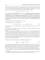
CHAPTER 2. QUALITY OF INFORMATION 17
Phenomena
state
Information
quality
Quality
requirements
Sensor
selection
Selection
constraints
Resource
availability
Resource use
by applications
Set of
applications

System
events
Service
discipline
Factors
Goals
Figure 2.1: Diagram describing the dependency between factors affecting the
quality of information delivered to a consumer.
DC
d−u
= P (|z(t) −pz(t)| < ε | Z)
2.3 Information quality dependency
To tackle the problem of information quality assurance, we first need to
understand the factors on which the IQ of delivered information depends.
Figure 2.1 depicts the dependencies between different mechanisms existing
in sensor networks. In drawing these dependencies we assume a general
sensor network model with only one important assumption - that there is a
redundancy in the number of sensors and we have a choice of sensor to select
among all available to do the phenomena monitoring.
There are four major factors affecting the quality of information delivered
to a sensor network consumer
1. State of physical phenomena under consideration. This may in-
clude both the changes in the environment that affect the measured
values at sensors as well as the changes of sensor condition themselves
such as specifics of measuring modalities.
2. Sensor selection, that is, the choice of sensors participating in data
acquisition.
CHAPTER 2. QUALITY OF INFORMATION 18
3. Resources available on the sensor nodes for data acquisition, pro-
cessing or transmission.

4. Resource use by applications. In this category are included the
structure of an application, operator deployment on sensor nodes and
throughput characteristics of an application.
Omitted from the list are the factors which depend almost entirely on a
particular network configuration and which we cannot change such as topol-
ogy of sensor deployment.
There is a dependency between three of these factors. When the state
of phenomena changes, we would probably need to update the set of sensors
participating in the measurement because the current set may no longer give
satisfactory quality of information. The change in the set of participating
sensors leads to a change in resources available on individual sensors. This
change in resource availability, in turn, may affect the quality of information
delivered such that it is no longer satisfactory. Since we consider dynamic en-
vironment, we have to assume that all of these three factors are dynamic and
therefore we need to consider their overall effect on the IQ. Most important,
we have to include phenomena state awareness into the framework.
2.4 Conclusion
The definition of the IQ metrics allows us to build systems which use the
above definition to translate the underlying resources used into guarantees
on defined IQ metrics. It may not be possible to address all the possible IQ
metrics within one framework, since different levels of information have to
be considered.
In the next two chapters, we will introduce two frameworks which address
certain IQ metrics, the first one focused on the data level information, and
the second one on the high-level information.
Chapter 3
Data-level query
admission-control
A significant number of sensor networks simply collect data without process-
ing its content to extract meaning from the underlying semantic. Aggrega-

tion functions in this case are simple and easily computed, and sensors are
selected for the duration of the entire process of the data acquisition. Be-
low, we consider such a scenario to provide the IQ guarantees for distributed
sensor network queries. The contribution of this chapter is analytical solu-
tion for approximated distribution of delay and loss of aggregated data for
a tree-shaped sensor query, assuming that wireless MAC protocol uses ex-
ponential back-off in case of transmission errors. This approximation allows
control over data level IQ metrics of data completeness, data coherence and
coverage.
3.1 Introduction
Recent developments in sensor networks have made it possible to gather up-
to-date information about the environment, through SQL type queries [BW01]
that capture streams of aggregated information over long periods of time.
However, for this information to be useful it has to be timely and complete;
in other words, there has to be a preservation of bounds on the delay and
loss of data. These considerations constitute attributes of information quality
delivered by a sensor network [BNQP05, BDQ
+
05, LN00].
In the case of aggregated data being delivered to a consumer, (and this is
most often the case in sensor networks), instead of the ratio of delivered data
to sensor produced data, completeness may actually mean the ratio of data
that is used in producing the aggregated result delivered to the consumer, to
19