A modeling study of ion implantation in crystalline silicon involving monte carlo and molecular dynamics methods
Bạn đang xem bản rút gọn của tài liệu. Xem và tải ngay bản đầy đủ của tài liệu tại đây (13.46 MB, 305 trang )
A MODELING STUDY OF ION IMPLANTATION IN
CRYSTALLINE SILICON INVOLVING MONTE CARLO
AND MOLECULAR DYNAMICS METHODS
CHAN HAY YEE, SERENE
NATIONAL UNIVERSITY OF SINGAPORE
2006
A MODELING STUDY OF ION IMPLANTATION IN
CRYSTALLINE SILICON INVOLVING MONTE CARLO
AND MOLECULAR DYNAMICS METHODS
CHAN HAY YEE, SERENE
{B. Eng (Hons.), NUS}
A THESIS SUBMITTED
FOR THE DEGREE OF DOCTOR OF PHILOSOPHY
DEPARTMENT OF CHEMICAL AND BIOMOLECULAR
ENGINEERING
NATIONAL UNIVERSITY OF SINGAPORE
2006
i
ACKNOWLEDGEMENT
I wish to thank my main supervisor, Associate Professor Srinivasan M.P for his patience and
guidance in my doctoral work at the National University of Singapore. Without him and the
support of the Chemical and Biomolecular Engineering department, this work would not have
progressed as smoothly as it had. I would also like to thank my past and present co-supervisors,
Dr Ida Ma Nga Ling and Dr Jin Hongmei from the Institute of High Performance Computing
for all resources, encouragement and invaluable discussions. I would also like to express
heartfelt gratitude to my mentors at Chartered Semiconductor, Dr Lap Chan, Dr Ng Chee
Mang and Dr Francis Benistant for all computational and fab equipment resources and for
imparting their vast knowledge in all aspects. Their constant support and enthusiasm provided
light at the tunnel’s end in an otherwise dreary path.
This work would not have possible without the support from a few research institutes and
organizations, namely Axcelis Technologies (U.S), Cascade Scientific (U.K), Integrated
Systems Engineering (ISE, Zurich), Institute of Materials Research and Engineering (IMRE,
Singapore), Institute of High Performance Computing (IHPC, Singapore) and the department
of Physics (NUS, Singapore). My scholarship from the Agency of Science, Technology and
Research (A*STAR, Singapore) is also gratefully acknowledged.
I wish to express my appreciation to my fellow friends in NUS and colleagues in Chartered
Special Projects group for all fun and laughter, peace and joy. Lastly, I would like to express
my love and gratitude to my parents who have been standing beside me all these years, and my
brother who never thought I would come this far. And of course to the special person in my
life, John, for holding my hand through the trials and tribulations.
ii
TABLE OF CONTENTS
Contents Page
Title page
Acknowledgements i
Table of contents ii
Summary vi
List of Tables viii
List of Figures xi
List of Symbols xviii
Chapter 1 INTRODUCTION 1
1.1 Motivation 1
1.2 Dissertation objectives 4
1.3 Dissertation overview 5
Chapter 2 BACKGROUND LITERATURE 6
2.1 Modeling ion implantation 6
2.1.1 Analytical distribution functions 6
2.1.2 Atomistic models: Monte Carlo and Molecular Dynamics methods 11
2.2 Energy loss mechanisms in solids 22
2.2.1 Nuclear energy loss 25
2.2.2 Electronic energy loss 29
2.3 Experimental techniques for range profiling 34
2.3.1 Ion implantation 34
2.3.2 Impurity depth profiling 37
iii
Chapter 3 METHODOLOGY I: MONTE CARLO METHODS 41
3.1 Theory of Binary Collision Approximation (BCA) 41
3.2 Monte Carlo BCA code Crystal-TRIM 47
3.2.1 Nuclear energy loss: ZBL universal potential 48
3.2.2 Electronic energy loss: ZBL and Oen-Robinson model 53
3.2.3 Damage accumulation model 61
3.2.4 Statistical enhancement techniques 64
3.2.4.1 Trajectory splitting 64
3.2.4.2 Lateral replication 65
3.2.4.3 Statistical reliability check 66
3.3 Input parameters to the Crystal-TRIM code 67
Chapter 4 NEW ION IMPLANTATION MODEL 71
4.1 Limitations of current analytical methods 71
4.1.1 Gaussian (Normal) distribution 71
4.1.2 Pearson IV and dual-Pearson IV distribution 73
4.1.3 Legendre polynomials 79
4.2 Sampling calibration of profiles (SCALP) 82
4.3 Assimilation of SCALP tables in process simulators 95
Chapter 5 METHODOLOGY II: MOLECULAR DYNAMICS METHODS 99
5.1 Theory of Molecular Dynamics (MD) 99
5.1.1 Integration algorithm 101
5.1.2 Interatomic potentials and force calculations 103
5.1.3 Boundary and initial state conditions 104
5.1.4 Acceleration methods 107
5.1.4.1 Neighbor list method 107
iv
5.1.4.2 Linked cell or cellular method 108
5.1.4.3 Variable time step method 108
5.2 Molecular dynamics code MDRANGE 109
5.2.1 Initial and boundary conditions 109
5.2.2 Nuclear energy loss: First principles potential 111
5.2.2.1 Density functional theory 112
5.2.2.2 Atomic basis sets 113
5.2.2.3 Single-point energy calculations 115
5.2.3 Electronic energy loss: PENR model 117
5.2.4 Damage accumulation model 124
5.2.5 Statistical enhancement techniques 128
Chapter 6 APPLICATION OF MOLECULAR DYNAMICS IN ION
IMPLANTATION 131
6.1 First-principle studies of BCA breakdown 132
6.2 SIMS database (intermediate to high energy) 135
6.3 Simulation of range profiles using MD 136
6.3.1 Effect of interatomic potential: ZBL versus DMOL 137
6.3.2 Effect of electronic stopping model: ZBL versus PENR 143
6.4 Comparisons of experiments with simulation (high energy) 147
Chapter 7 EXPERIMENTAL VERIFICATION AND CALIBRATION 152
7.1 Quantitative analysis of Secondary Mass Ion Spectrometry (SIMS) 152
7.2 SIMS database (low to intermediate energy) 156
7.3 Comparisons of experiments with simulation (low energy) 163
7.4 Further SIMS study: different techniques and instruments 176
7.4.1 Use of other mass analyzers 176
v
7.4.2 Equipment capabilities and limitations 186
Chapter 8 SUMMARY OF WORK 191
8.1 Major contributions of present work 191
8.2 Recommendations for future work: Diffusion studies 197
8.2.1 Diffusion-limited reaction model and simulation method 198
8.2.2 Theoretical diffusion model 199
8.2.3 Spatially uniform point defect distributions 200
8.2.4 Spatially variant point defect distributions 204
Chapter 9 CONCLUSIONS 208
REFERENCES 210
APPENDICES 227
Appendix A Mathematical formulation of other electronic stopping models 227
Appendix B Tabulated data of SCALP coefficients for B, P, Ge, As, In and Sb 232
Appendix C C++ program codes for extraction of SCALP coefficients 251
Appendix D DMOL input files used in potential calculations 259
Appendix E Mathematical formulation of scattering phaseshifts 275
CURRICULUM VITAE 280
vi
SUMMARY
The modeling of ion implantation profiles has been a longstanding problem. From the initial
use of analytical functions based on empirical parameters to the use of atomistic methods to
predict the dopant distributions, countless problems have been faced and addressed. Each
passing generation in the growth of the integrated-circuit chip demands smaller feature
dimensions and shallower source drain junctions. Modeling techniques based on continuum
methods are no longer sufficient to address problems based on an atomistic scale.
In this dissertation, the limitations faced by common analytical models of ion implantation are
addressed. Atomistic methods are deemed to replace such statistically-based methods. Monte
Carlo and molecular dynamics are the two main techniques used. Such methods are physically
realistic and the implementation of these methods is no longer hindered by long computational
times and insufficient memory space with the advent of supercomputers. A new ion
implantation model is proposed in this thesis that not only combines the simplicity of
analytical techniques, but also the accuracy of atomistic methods. It can also be easily
assimilated in commercial process simulators for two/three-dimensional simulation and
diffusion studies. Based on this new model and extensive Monte Carlo simulations,
implantation tables are set up and presented. However, typical Monte Carlo methods are based
on the binary collision approximation (BCA) which becomes inaccurate at low implant
energies. The exact breakdown energies have never been clearly defined; this work attempts to
estimate these energies for different dopants from first-principles calculations.
Molecular dynamics is proposed to replace Monte Carlo methods in the low energy regime.
Not only are multiple interactions accounted for, the molecular dynamics code used in this
work allows for the use of accurate interatomic potentials calculated specifically for each ion-
target pair. The potentials are calculated from density functional theory and found to give
substantially improved results over commonly used repulsive potentials. The electronic losses
vii
associated with each collision are also accurately predicted by the use of a robust local
electronic stopping model based on phase shift factors. The phase shifts are calculated from
first-principles scattering theory and found to give accurate range profiles even in channeling
directions. A low energy database consisting of a large number of experimentally measured
profiles have been set up not only to verify the models in the codes, but also to identify and
eliminate common experimental artifacts associated with ultra-shallow depth profiling.
Different SIMS (Secondary Ion Mass Spectrometry) instruments have been used at optimized
analyzing conditions in the setting up of this database. By comparing simulation and
experiments, the capabilities and limitations of different mass analyzers have been ascertained.
A technique has also been proposed to utilize the ranges of coincidences between simulated
and experimental profiles to calibrate the full low energy profile. The comparisons also show
that the BCA breakdown limits are reasonable approximations to the true limits.
This work yields not only a reproducible method to model ion implantation profiles; in
addition, well-calibrated simulated and experimental ultra-shallow profiles have been obtained
which serve to provide a good foundation for future diffusion studies. Not only does this work
have an important impact on future device modeling, it possesses useful applications in the
semiconductor industry, especially since feature miniaturization demands accurate modeling of
implantation profiles. This work answers the necessary call for the scaling of technology nodes
and provides a good foundation for advances in TCAD simulation.
viii
LIST OF TABLES
Table Description Page
4.1 Parameters for mean projected range 76
4.2 Parameters for vertical standard deviation 76
4.3 Parameters for vertical skewness 76
4.4 Parameters for vertical kurtosis 77
4.5 Functional forms of the first 14 Legendre polynomials 79
4.6 Tabulated SCALP coefficients for (a) impurity (b) interstitial (c) vacancy profiles.
B 1-100keV, 1×10
13
atoms/cm
2
, 7°
tilt and 22° rotation 89
4.7 Prediction of impurity profile at 15keV by direct interpolation between 10 and
20keV (a) Interpolated Tdepth and Cx% values shown in bold (b) Reconstruction
of desired profile by reverse SCALP method 91
5.1 Phase shifts obtained from DFT calculation for B using the code jellium from (a)
l=0 to l=7 for r
S
up to 1.0 only and (b) l=8 to l=10, including calculations for
electron density ρ, Fermi momentum k
F
and the final electronic stopping
(Q*conversion factor) 121
6.1 Estimated energy limits (keV) below which BCA breaks down 132
6.2 SIMS database (intermediate to high energy): range of implant conditions 135
7.1 Implant conditions for 72-wafer split involving nine species 158
8.1 Forward and backward reaction rates in diffusion model 196
B.1 Amorphization threshold for six different species (B, P, Ge, As, In and Sb) 229
B.2 SCALP coefficients for B (a) impurity (b) interstitial (c) vacancy for energies 1 to
100keV at dose 1×10
13
atoms/cm
2
and tilt 7° rotation 22° 230
ix
B.3 SCALP coefficients for B (a) impurity (b) interstitial (c) vacancy for energies 1 to
100keV at dose 1×10
13
atoms/cm
2
and tilt 0° rotation 0° 231
B.4 SCALP coefficients for B (a) impurity (b) interstitial (c) vacancy for energies 1 to
100keV at dose 1×10
13
atoms/cm
2
and tilt 45° rotation 45° 232
B.5 SCALP coefficients for P (a) impurity (b) interstitial (c) vacancy for energies 1 to
100keV at dose 1×10
13
atoms/cm
2
and tilt 7° rotation 22° 233
B.6 SCALP coefficients for P (a) impurity (b) interstitial (c) vacancy for energies 1 to
100keV at dose 1×10
13
atoms/cm
2
and tilt 0° rotation 0° 234
B.7 SCALP coefficients for P (a) impurity (b) interstitial (c) vacancy for energies 1 to
100keV at dose 1×10
13
atoms/cm
2
and tilt 45° rotation 45° 235
B.8 SCALP coefficients for Ge (a) impurity (b) interstitial (c) vacancy for energies 1
to 100keV at dose 1×10
13
atoms/cm
2
and tilt 7° rotation 22° 236
B.9 SCALP coefficients for Ge (a) impurity (b) interstitial (c) vacancy for energies 1
to 100keV at dose 1×10
13
atoms/cm
2
and tilt 0° rotation 0° 237
B.10 SCALP coefficients for Ge (a) impurity (b) interstitial (c) vacancy for energies 1
to 100keV at dose 1×10
13
atoms/cm
2
and tilt 45° rotation 45° 238
B.11 SCALP coefficients for As (a) impurity (b) interstitial (c) vacancy for energies 1
to 100keV at dose 1×10
13
atoms/cm
2
and tilt 7° rotation 22° 239
B.12 SCALP coefficients for As (a) impurity (b) interstitial (c) vacancy for energies 1
to 100keV at dose 1×10
13
atoms/cm
2
and tilt 0° rotation 0° 240
B.13 SCALP coefficients for As (a) impurity (b) interstitial (c) vacancy for energies 1
to 100keV at dose 1×10
13
atoms/cm
2
and tilt 45° rotation 45° 241
B.14 SCALP coefficients for In (a) impurity (b) interstitial (c) vacancy for energies 1
to 100keV at dose 1×10
13
atoms/cm
2
and tilt 7° rotation 22° 242
B.15 SCALP coefficients for In (a) impurity (b) interstitial (c) vacancy for energies 1
to 100keV at dose 1×10
13
atoms/cm
2
and tilt 0° rotation 0° 243
x
B.16 SCALP coefficients for In (a) impurity (b) interstitial (c) vacancy for energies 1
to 100keV at dose 1×10
13
atoms/cm
2
and tilt 45° rotation 45° 244
B.17 SCALP coefficients for Sb (a) impurity (b) interstitial (c) vacancy for energies 1
to 100keV at dose 1×10
13
atoms/cm
2
and tilt 7° rotation 22° 245
B.18 SCALP coefficients for Sb (a) impurity (b) interstitial (c) vacancy for energies 1
to 100keV at dose 1×10
13
atoms/cm
2
and tilt 0° rotation 0° 246
B.19 SCALP coefficients for Sb (a) impurity (b) interstitial (c) vacancy for energies 1
to 100keV at dose 1×10
13
atoms/cm
2
and tilt 45° rotation 45° 247
D.1 Input parameters in .inatom file for nine species (B, C, N, F, P, Ge, As, In and Sb)
and Si as target, with standard DN basis sets and additional hydrogenic orbitals
271
xi
LIST OF FIGURES
Figure Description Page
1.1 (a) Structure of an Metal Oxide Semiconductor (MOS) device 1
(b) Cross-sectional view of MOS device
2.1 Schematic of a commercial ion implanter 36
2.2 Principles of Secondary Ion Mass Spectrometry 38
2.3 Quadrupole mass analyzer consisting of four circular rods
(a) Front view
(b) Cross sectional view 39
3.1 Schematic drawing of two-body scattering theory in laboratory coordinates 41
3.2 Schematic drawing of two-body scattering theory in center-of-mass
coordinates 43
3.3 Angular conversion of center-of-mass coordinates to laboratory coordinates
for the (a) target particle and (b) projectile particle 43
3.4 Energies (in eV) obtained from the ZBL universal potential function for
nine dopants (B, C, N, F, P, Ge, As, In and Sb) 51
3.5 Universal nuclear stopping in eV/atom/cm
2
for nine dopants
(B, C, N, F, P, Ge, As, In and Sb) 52
3.6 ZBL electronic stopping in eV/atom/cm
2
for nine dopants
(B, C, N, F, P, Ge, As, In and Sb) 58
3.7 Relative importance of nuclear (ZBL) and electronic (ZBL) stopping for B
and Sb in different energy regimes 59
3.8 Different electronic stopping models compared against the non-local ZBL
model for B only 60
3.9 Effect of enhanced dechanneling on profile shape for (a) B 100keV (b) Sb
100keV 7° tilt 22° rotation, doses 1×10
12
-1×10
15
atoms/cm
2
63
xii
3.10 Choice of interval width, w on final simulated impurity profile. All simulated
results are obtained from Crystal-TRIM Version 98F/1D,3D for B 1keV 1×10
13
atoms/cm
2
0° tilt 0° rotation using (a) w = 30Å (b) w=2Å and (c) w=7Å 69
4.1 Logarithmic Gaussian function with D
T
= 1 × 10
13
atoms/cm
2
(a) different Rp,
constant σ
z
(0.005µm) and (b) different σ
z
, constant Rp (0.01µm) 71
4.2 Gaussian fits to SIMS profiles (a) As 2keV, 5keV 5 × 10
14
atoms/cm
2
tilt 0°
rotation 0° and (b) Sb 50keV, 100keV 1 × 10
13
atoms/cm
2
tilt 0° rotation 0° 71
4.3 Experimental SIMS and simulated profiles in crystalline and amorphous Si (a) B
500eV 5×10
14
atoms/cm
2
and As 5keV 1×10
15
atoms/cm
2
at 0°
tilt and 0° rotation
(b) P 20keV 1×10
15
atoms/cm
2
and Sb 100keV 1×10
13
atoms/cm
2
at 7°
tilt and 22°
rotation 73
4.4 Comparisons between Hobler’s fitting formulae (10-300keV) and extracted
Pearson IV moments from Crystal TRIM simulated profiles (100eV-300keV) for 3
different tilts/rotations, 7°/22°, 0°/0° and 45°/45° in single-crystalline silicon (a)
mean projected range (b) standard deviation (c) skewness (d) kurtosis with implant
energy, E 74
4.5 (a) 3D trajectories of each implanted ion and their recoils. The inset in (a) shows
the low channeling 7°/22° implant. (b) Extracted 1D impurity profiles in vertical
direction 75
4.6 Random trends of the Legendre coefficients (a
5
, a
10
and a
15
) with implant energies.
Implant conditions: B in Si 1-100keV 1e13atoms/cm
2
7
0
tilt 22
0
rotation 79
4.7 Instability of the fitted profiles with increasing order of Legendre polynomials.
Implant conditions: B in Si 1-100keV 1e13atoms/cm
2
7
0
tilt 22
0
rotation 80
4.8 Comparison of experimental SIMS data and simulation for B 0.5keV 1×10
15
atoms/cm
2
0°
tilt and 0° rotation and 10keV 1×10
15
atoms/cm
2
0°
tilt and 0°
rotation 82
4.9 Comparison of experimental SIMS data and simulation for C 0.5keV 1×10
14
atoms/cm
2
0°
tilt and 0° rotation and 2keV 1×10
14
atoms/cm
2
45°
tilt and 45°
rotation 82
4.10 Comparison of experimental SIMS data and simulation for N 3keV 1×10
14
atoms/cm
2
7°
tilt and 22° rotation and 15keV 1×10
15
atoms/cm
2
5.2°
tilt and 17°
rotation 83
xiii
4.11 Comparison of experimental SIMS data and simulation for F 1keV 6×10
13
atoms/cm
2
0°
tilt and 0° rotation and 5keV 6×10
13
atoms/cm
2
45°
tilt and 45°
rotation 83
4.12 Comparison of experimental SIMS data and simulation for P 1keV 5×10
13
atoms/cm
2
0°
tilt and 0° rotation and 5keV 5×10
13
atoms/cm
2
45°
tilt and 45°
rotation 84
4.13 Comparison of experimental SIMS data and simulation for Ge 5keV 5×10
13
atoms/cm
2
45°
tilt and 45° rotation and 30keV 5×10
13
atoms/cm
2
5.2°
tilt and 17°
rotation 84
4.14 Comparison of experimental SIMS data and simulation for As 5keV 1×10
15
atoms/cm
2
0°
tilt and 0° rotation and 10keV 5×10
13
atoms/cm
2
0°
tilt and 0°
rotation 85
4.15 Comparison of experimental SIMS data and simulation for In 10keV 5×10
13
atoms/cm
2
45°
tilt and 45° rotation and 40keV 2×10
13
atoms/cm
2
7°
tilt and 27°
rotation 85
4.16 Comparison of experimental SIMS data and simulation for Sb 10keV 5×10
13
atoms/cm
2
45°
tilt and 45° rotation and 100keV 1×10
13
atoms/cm
2
7°
tilt and 27°
rotation 86
4.17 Graphical representation of the SCALP technique. Cutoff concentration of 1×10
15
atoms/cm
3
is used. Cx% refers to the concentration at x% of Tdepth 88
4.18 Correlation of (a) C0%, C5% and (b) C90%, C95% with implant energy. Implant
conditions are the same as for Table 4.6. Power law (y=ax
b
) coefficients for 7°/22°
are a=2.8113×10
18
, b=-1.05791 90
4.19 Interpolated 30keV interstitial profile against simulated profile 91
4.20 Modeling of impurity profiles with SCALP coefficients (P 60keV, 80keV and
100keV, 1×10
13
atoms/cm
2
at 45° tilt and 45° rotation) 92
4.21 Modeling of interstitial profiles with SCALP coefficients (Sb 15keV, 30keV and
50keV, 1×10
13
atoms/cm
2
at 0° tilt and 0° rotation) 93
4.22 Modeling of vacancy profiles with SCALP coefficients (As 60keV, 80keV and
100keV, 1×10
13
atoms/cm
2
at 45° tilt and 45° rotation) 93
xiv
4.23 Lateral spreading accounted for by specification of σ
LAT
in DIOS 95
4.24 Vertical and lateral standard deviation for As 0.1-100keV, 5×10
14
atoms/cm
2
at
7°/22, 0°/0° and 45°/45°. 95
4.25 Vertical impurity profile obtained by one-dimensional cut (Fig. 4.23) at x=0.8µm.
SIMS data is shown for comparison (As in Si 10keV, 5×10
14
atoms/cm
2
0° tilt 0°
rotation) 96
5.1 Simplified flowchart depicting MD algorithm 99
5.2 Schematic diagram of MD simulation of thermal motion for 100 time steps
(Courtesy of lecture notes from K. Nordlund) 100
5.3 Schematic of two-dimensional periodic boundary condition 104
5.4 Schematic of the neighbor-list or book-keeping method. Time for usual potential
calculations reduced from Θ(N
2
) to Θ(N) 106
5.5 Schematic of linked cell method 107
5.6 Schematic two-dimensional view of cell translation technique (a) before and (b)
after ion movement 110
5.7 Energies (in eV) obtained from DFT calculations utilizing the DMOL package for
nine dopants (B, C, N, F, P, Ge, As, In and Sb) 115
5.8 Algorithm for calculation of Q and scattering phaseshifts 119
5.9 Fermi surface value Q versus one-electron radius, r
S
for nine dopant systems (a) B,
F and As (b) C, P and In (c) N, Ge and Sb. Multiplication of Q by the ion velocity
gives the electronic stopping power 121
5.10 Schematic of the damage accumulation model 123
5.11 Effect of enhanced dechanneling and damage accumulation on profile shape for (a)
B 100keV 7° tilt 22° rotation and (b) Sb 100keV 7° tilt 22° rotation for doses
1×10
12
-1×10
15
atoms/cm
2
124
xv
5.12 Impurity files of B and Sb at dose 1×10
15
atoms/cm
2
obtained from Crystal-TRIM
and MDRANGE 125
5.13 REED algorithm for generating splitting depths from the integrals of initial profile,
with weights associated with split ions at each depth 127
5.14 Comparison of experimental SIMS data and simulation for In 40keV, 2×10
13
atoms/cm
2
7°
tilt and 27° rotation with and without REED algorithm 127
6.1 Correlation of BCA breakdown limits calculated by DFT with atomic mass (power
law) and atomic number (linear) 133
6.2 Energies (in eV) obtained from DFT calculations utilizing the DMOL package for
(a) B and Sb (b) C, P and In 134
6.3 (a) ZBL and DMOL potentials for B-Si and As-Si systems (b) MD simulated
profiles of B and As in Si (200eV 1×10
13
atoms/cm
2
7° tilt and 22° rotation) using
potentials in (a) 137
6.4 Comparison of experimental SIMS and MD simulation (ZBL versus DMOL
potential) for B (a) 0.5keV 5×10
13
atoms/cm
2
45° tilt and 0° rotation (b) 10keV
1×10
15
atoms/cm
2
0° tilt and 0° rotation 140
6.5 Comparison of experimental SIMS and MD simulation (ZBL versus DMOL
potential) for As (a) 1keV 1×10
15
atoms/cm
2
5.2° tilt and 17° rotation (b) 10keV
5×10
14
atoms/cm
2
0° tilt and 0° rotation 141
6.6 Comparison of experimental SIMS and MD simulation (ZBL versus PENR
electronic stopping) for N (a) 0.5keV 1×10
14
atoms/cm
2
0° tilt and 0° rotation (b)
15keV 1×10
15
atoms/cm
2
5.2° tilt and 17° rotation 144
6.7 Comparison of experimental SIMS and MD simulation (ZBL versus PENR
electronic stopping) for Sb (a) 10keV 5×10
13
atoms/cm
2
45° tilt and 45° rotation (b)
50keV 3.85×10
13
atoms/cm
2
30° tilt and 0° rotation 145
6.8 Comparison of experimental SIMS data and MD simulation for B 5keV 5×10
14
atoms/cm
2
0°
tilt and 0° rotation and 10keV 1×10
15
atoms/cm
2
0°
tilt and 0°
rotation 148
6.9 Comparison of experimental SIMS data and MD simulation for Ge 30keV 1×10
14
atoms/cm
2
5.2°
tilt and 17° rotation and 50keV 1×10
14
atoms/cm
2
5.2°
tilt and 17°
rotation 149
xvi
6.10 Comparison of experimental SIMS data and MD simulation for As 30keV 1×10
15
atoms/cm
2
7°
tilt and 23° rotation and 50keV 1×10
15
atoms/cm
2
7°
tilt and 23°
rotation 149
6.11 Comparison of experimental SIMS data and MD simulation for In 40keV 2×10
13
atoms/cm
2
7°
tilt and 27° rotation and 100keV 1×10
14
atoms/cm
2
0°
tilt and 0°
rotation 150
6.12 Comparison of experimental SIMS data and MD simulation for Sb 50keV
4.14×10
13
atoms/cm
2
30°
tilt and 18° rotation and 100keV 1×10
14
atoms/cm
2
0°
tilt
and 0° rotation 150
7.1 RSF values for all stable elements measuring (a) positive secondary ions with O
+
primary beam and (b) negative secondary ions with Cs
+
primary beam 154
7.2 Comparison of experimental SIMS and simulation (BCA versus MD) for B (a)
0.5keV 5×10
13
atoms/cm
2
45° tilt and 0° rotation (b) 0.5keV 5×10
13
atoms/cm
2
45°
tilt and 18° rotation 162
7.3 Comparison of experimental SIMS and simulation (BCA versus MD) for C (a)
1keV 1×10
14
atoms/cm
2
45° tilt and 45° rotation (b) 2keV 1×10
14
atoms/cm
2
0° tilt
and 0° rotation 163
7.4 Comparison of experimental SIMS and simulation (BCA versus MD) for N (a)
0.5keV 1×10
14
atoms/cm
2
0° tilt and 0° rotation (b) 2keV 1×10
14
atoms/cm
2
45°
tilt and 45° rotation 164
7.5 Comparison of experimental SIMS and simulation (BCA versus MD) for F (a)
1keV 6×10
13
atoms/cm
2
45° tilt and 45° rotation (b) 5keV 6×10
13
atoms/cm
2
45°
tilt and 45° rotation 165
7.6 Comparison of experimental SIMS and simulation (BCA versus MD) for P (a)
1keV 5×10
13
atoms/cm
2
0° tilt and 0° rotation (b) 2keV 5×10
13
atoms/cm
2
0° tilt
and 0° rotation 166
7.7 Comparison of experimental SIMS and simulation (BCA versus MD) for As (a)
2keV 5×10
13
atoms/cm
2
45° tilt and 45° rotation (b) 5keV 5×10
13
atoms/cm
2
0° tilt
and 0° rotation 167
7.8 Comparison of experimental SIMS and simulation (BCA versus MD) for Ge (a)
3keV 5×10
13
atoms/cm
2
0° tilt and 0° rotation (b) 5keV 5×10
13
atoms/cm
2
0° tilt
and 0° rotation 168
xvii
7.9 Comparison of experimental SIMS and simulation (BCA versus MD) for In (a)
2keV 5×10
13
atoms/cm
2
45° tilt and 45° rotation (b) 10keV 5×10
13
atoms/cm
2
0°
tilt and 0° rotation 169
7.10 Comparison of experimental SIMS and simulation (BCA versus MD) for Sb (a)
5keV 1×10
14
atoms/cm
2
7° tilt and 22° rotation (b) 10keV 5×10
13
atoms/cm
2
45°
tilt and 45° rotation 170
7.11 Comparison of SIMS (Q, MS and ToF) for As
(a) 2keV 5×10
13
atoms/cm
2
0° tilt and 0° rotation 176
(b) 2keV 5×10
13
atoms/cm
2
45° tilt and 45° rotation
(c) 5keV 5×10
13
atoms/cm
2
0° tilt and 0° rotation 177
(d) 5keV 5×10
13
atoms/cm
2
45° tilt and 45° rotation
(e) 10keV 5×10
13
atoms/cm
2
0° tilt and 0° rotation 178
(f) 10keV 5×10
13
atoms/cm
2
45° tilt and 45° rotation
7.12 Comparison of SIMS (Q, MS(I), MS(II) and ToF) for P
(a) 1keV 5×10
13
atoms/cm
2
0° tilt and 0° rotation 180
(b) 1keV 5×10
13
atoms/cm
2
45° tilt and 45° rotation
(c) 2keV 5×10
13
atoms/cm
2
0° tilt and 0° rotation 181
(d) 2keV 5×10
13
atoms/cm
2
45° tilt and 45° rotation
(e) 5keV 5×10
13
atoms/cm
2
0° tilt and 0° rotation 182
(f) 5keV 5×10
13
atoms/cm
2
45° tilt and 45° rotation
7.13 Comparison of experimental SIMS and simulation (Q, MS(II), ToF versus MD)
for P 1keV 5×10
13
atoms/cm
2
0° tilt and 0° rotation 187
8.1 Concentration of (a) I and (b) V in clusters (N ≤ 10) at RT. Only clustering
reactions are included. Time evolution from 10
-10
- 10
7
s is shown 199
8.2 Distribution of (a) I and (b) V in clusters (N ≤ 50) at 850°C after different time
periods (1s and 10s). Only clustering reactions are included 201
8.3 Simulated impurity, damage (I and V) and net excess point defect concentrations
for 10keV As implant at dose 1×10
13
atoms/cm
2
into crystalline silicon 202
8.4 Plus factors calculated from remaining I concentrations (As 10keV, 1×10
13
atoms/cm
2
) after different diffusion periods using the Waite model and current
model 203
8.5 Plus factors calculated from remaining I concentrations (As 10keV, 1×10
13
atoms/cm
2
) after different diffusion periods using current model 204
xviii
LIST OF SYMBOLS
(
)
zC Number of ions per unit volume (concentration)
z Implanted depth taken in the vertical direction
T
D
Number of ions per unit area impacting on the wafer surface (dose)
p
R
Mean projected range
z
σ
Projected range straggling (vertical standard deviation)
LAT
σ
Projected range straggling (lateral standard deviation)
γ Skewness, third moment of Pearson IV distribution, accounts for asymmetry
β Kurtosis, fourth moment of Pearson IV distribution, accounts for flatness of profile
V(r) Interatomic potential between atoms/potential energy of system
a
0
Bohr radius (0.529Å)
a Screening parameter
r Interatomic distance between atoms
r
C
Cut-off radius, maximum distance where surrounding atom affects the central atom
∆r Infinitesimal displacement of atoms
t
0
Initial time
t Instantaneous time
∆t Infinitesimal time step
Z
1
Atomic number of projectile (implanted ion)
E
0
Initial energy of incident ion
M
1
Atomic mass of projectile (implanted ion)
V
0
Incident velocity of projectile ion
V
1
Projectile ion’s final velocity
Z
2
Atomic number of target (substrate atom)
M
2
Atomic mass of target atom (substrate atom)
xix
V
2
Target atom’s final velocity
E
C
Total energy of system in center-of-mass (CM) coordinates
M
C
Mass of projectile ion in center-of-mass (CM) coordinates
V
C
Velocity of projectile ion in center-of-mass (CM) coordinates
φ Angle of recoil after impact in laboratory coordinates
Φ Angle of recoil after impact in center-of-mass (CM) coordinates
Θ Final angle of scatter after impact in center-of-mass (CM) coordinates
J
C
Angular momentum in center-of-mass (CM) coordinates
P Impact parameter
T Energy transferred in the collision from incident projectile to target projectile
ε Reduced energy
S Stopping energy in units of eV/atom/cm
2
Z
eff
Effective charge of projectile ion
γ Correction factor relating effective charge to Z
1
ν Instantaneous velocity of projectile ion
ν
r
Instantaneous velocity of the ion relative to the electrons
ν
F
Fermi velocity of target electrons
y
r
Reduced relative velocity of projectile ion
ρ Electron density
r
s
One-electron radius of a centrosymmetric electron charge distribution
Λ Screening length which describes how electrons screen the nucleus
N Number of electrons bound to the ion
q Charge fraction
R
0
Distance of closest approach in a binary collision
C
el
Parameters for local electronic energy loss in modified Oen-Robinson model
P
d
Probability that in a certain depth interval of the target a pseudo-projectile is moving in
a damaged region
xx
P
s
Saturation level of sub-linear growth or critical value for onset of super-linear increase
of the damage.
f
d
Damage accumulation function (dependent on defect types present)
A
n
E
Nuclear energy deposition per target atom
A
d
N Number of displacements per target atom
E
d
Displacement energy of silicon (~15eV)
L
i
Legendre polynomials of degree i
z
min
Minimum depth between which the impurity/damage concentration falls within the
range of interest
z
max
Maximum depth between which the impurity/damage concentration falls within the
range of interest
Tdepth Depth in µm where concentration is 1×10
15
atoms/cm
3
(used in SCALP model)
Cx% Concentration at x% of Tdepth (used in SCALP model)
z,y,x
∇
Gradient (del) in x-, y- and z- dimensions
F Interatomic force between atoms
k
B
Boltzmann constant 1.38066×10
-23
J/K
ψ Electron wavefunction
φ Molecular orbitals
χ
Atomic orbitals
k
F
Fermi momentum of target electrons
δ
l
Phaseshift for the scattering of an electron
E
F
Fermi energy
CHAPTER 1 1
CHAPTER 1 INTRODUCTION
1.1 Motivation
The main driving force for performance in the semiconductor industry lies in the need to
increase both the speed and the density of silicon transistors with decreasing size. Down-
scaling of transistor chip dimensions equates to larger numbers of devices per wafer, which
leads to higher performance, as smaller channel lengths result in faster transistors. Hence, for
similar processing costs, manufacturers can produce larger numbers of dies from the wafer or
improve the functionality of the chips by placing more transistors in the same die area. At
present, the semiconductor industry faces tough challenges in meeting its goal. The 2004
International Technology Roadmap for Semiconductors (ITRS) has highlighted the need for
characterization methodologies for ultra-shallow geometries, source-drain junctions and low
dopant levels. The main goal is to meet vertical junction depth prediction accuracy of 10% (of
the physical gate length) which falls approximately in the range of 2 to 4 nm. A schematic of
the Metal-Oxide Semiconductor (MOS) is given in Fig. 1.1 (Wolf, 1990).
Fig. 1.1 (a) Structure of an Metal-Oxide Semiconductor (MOS) device (b) Cross-sectional
view of MOS device
Typical silicon processing techniques include diffusion, ion implantation, oxidation, thin film
deposition, chemical or plasma etching, and metallization etc. Among all these processes, ion
implantation and dopant diffusion are particularly strongly affected by device miniaturization
and remains an active area of study. Ion implantation has been a dominant tool for introducing
dopants into the silicon crystal. A typical Complementary-MOS (CMOS) process employs
approximately a dozen ion implantation steps to form isolation wells, source/drain junctions,
(a)
(b)
CHAPTER 1 2
channel-stops, threshold voltage adjusts, punchthrough stoppers and other doped areas of the
p- and n-channel MOS transistors. Understanding key thermodynamic and transport
phenomena in the implant and diffusion steps with size shrinkage becomes increasingly
important, but increasingly difficult to study by experimental techniques alone. Moreover, the
cost of fabrication for test lots increases with each technology generation making
characterization of material parameters by the usual trial and error method extremely
expensive. These factors make simulation of front-end processes a critical component in
today’s integrated-circuit (IC) technology development. With the advent of faster and cheaper
supercomputers, simulation is not only an effective and affordable tool for exploring the
vertical and lateral profiles of a modern transistor; it aims to replace physical optimization
experiments with virtual ones.
The importance of predictive and computationally efficient implant and diffusion models for
the IC fabrication process is evident. As the ion enters the crystal, it gives up its kinetic energy
to the lattice atoms by means of nuclear stopping and electronic stopping and finally comes to
rest at some depth in the crystal. In order to accurately model the ion implantation process,
physically realistic models for both key stopping processes are essential. In addition,
implantation produces damage in the form of lattice point defects like interstitials and
vacancies, as well as non-substitutional dopants which destroys the pristine condition of
crystalline silicon. The induced damage causes dechanneling of the dopant and affects the
overall shape of the doping distribution, so an accurate impurity profile cannot be obtained
without correctly accounting for dechanneling effect of the damage. Moreover, most of the as-
implanted impurities are in interstitial sites and are thus electrically inactive. This necessitates
a high-temperature anneal step to activate the dopants atoms and repair the damaged silicon
crystal to maintain good electrical properties. Since dopant diffusion is mediated by point
defects and the number of such defects increases significantly after ion implantation, post
implant annealing is characterized by anomalous diffusion of dopants. This phenomenon,
CHAPTER 1 3
known as Transient Enhanced Diffusion (TED), results in junction depth changes and
degradation in the performance of advanced generation transistors. Right after the implantation
step, before the high temperature annealing, dopant atoms are already believed to interact with
point defects, forming mobile dopant-defect pairs, immobile complexes, and precipitates at
room temperature. At the same time, they may also undergo clustering, recombination and
diffusion processes. The final dopant distribution is thus a complex combination of a wide
range of atomic-scale interaction. Since TED is directly correlated with the implantation
impurity and damage distributions, accurate profiles are needed from the ion implantation
simulation to be the inputs for the diffusion simulations.
Ion implantation simulations can be broadly classified into three categories: one uses
phenomenological models, such as SUPREM IV (Law et al., 1988); the second one is based on
the binary collision approximation (BCA) such as in UT-MARLOWE (Tasch et al., 1989) and
Crystal-TRIM (Posselt et al., 1994), which are often referred to as Monte Carlo (MC)
simulators due to the use of random numbers; the final category is molecular dynamics (MD)
(Nordlund 1995). The last two categories are physically based methods, because the motion of
the particles is calculated using physical principles. Compared with the semi-empirical
phenomenological models, physically based models are rather computationally intensive,
however they compensate by their better predictive power. Under the binary collision
approximation, the motion of randomly generated energetic particles is described by sequences
of binary collisions with target atoms, and the energy loss and direction change at every
collision event are tracked. MD, on the other hand, describe the motion of all the atoms
concerned in the collision process, by establishing and solving numerically Newton’s equation
of motion for all the atoms in the system. The concept of MD is simple but requires longer
computational time and larger memory resources compared to MC methods based on BCA.
However, MD simulations can provide atomic and structural information which is not possible
by other methods, such as channeling effect, and time and space evolution of atomic