DESIGN AND CONTROL OF AUTONOMOUS MOBILE ROBOTS WITH IMPROVED DYNAMIC STABILITY 1
Bạn đang xem bản rút gọn của tài liệu. Xem và tải ngay bản đầy đủ của tài liệu tại đây (7.73 MB, 92 trang )
Chapter 1
Background and Literature Review
1.1 Mobile Wheeled Robot: A Historical Perspec-
tive
Most mobile machines and, particularly mobile robots, roll on wheels [1]. Although
legged and treaded locomotion were intensively studied and corresponding mobile
robots were developed in the last decade, it is commonly accepted that “wheeled
mobile robots are more energy-efficient than legged or treaded robots on hard, smooth
surface”[2]. Wheeled robots are mechanically simple and easy to construct. “Wheels
are simpler to control, pose fewer stability problems, use less energy per unit distance
of motion, and can go faster than legs”[3].
A definition of Wheeled Mobile Robot(WMR) found in [2] states: “A robot ca-
pable of locomotion on a surface solely through the actuation of wheel assemblies
mounted on the robot and in contact with the surface. A wheel assembly is a device
which provides or allows relative motion between its mount and a surface on which
it is intended to have a single point of rolling contact”.
1
WMR is classified according to the wheel arrangements as follows [1]:
• Differential Drive;
• Synchro Drive;
• Tricycle Drive Robot;
• Car-like Drive Robot;
A review and classifications of WMR with the aforementioned wheels were re-
ported in [2]. WMR with conventional and omni-directional wheel were analyzed in
[4]. In [5], the unified kinematics, both inverse and direct, is derived for four kinds of
wheeled vehicles: ordinary car-like robots (including passenger cars, single unit trucks,
single unit buses, and articulated trucks); dual drive robots (dual drive motors with
various casters); synchronous drive and steering robots; and omni-directional robots.
Rajagopalan [6] analyzed the kinematics of WMR with various combinations of-
driving and steering wheels. It was shown that for driverless ground vehicles (WMRs)
operating at low speed (<10 km/h) and not undergoing frequent accelerations and de-
celerations, the ”frictional effects are insignificant” and a kinematic model is sufficient.
On the other hand, Shekhar [7] proved that for fixed, centred, and omnidirectional
wheels, wheel slip is inevitable, for they cannot preserve the longitudinal (rolling
direction) constraints.
The most recent overview analysis of the development and classification of dif-
ferent kinds of wheeled mobile robots can be found in [1].
2
For all these kinds of mobile robots, the nonholonomic constraints reduce the
range of different motions allowed, thereby greatly complicating the motion planning
problem. In approaching this problem, different mechanisms for omni-directional
wheels have been developed in the past decades, namely, offset steered driving wheels;
omnidirectional wheels; spherical wheels: orthogonal-wheel assembly mechanisms;
spherical rob ots; ball-wheel omnidirectional mechanisms; etc. Vehicles with omnidi-
rectional wheels can freely move back, forth, and sideways or rotate in place.
Luca [8] and Murry [9] stated that nonholonomy usually rises from three different
sources:
1. Rolling Contacts without slip;
2. Conservation of angular Momentum in multibody systems;
3. Robotic devices under special control operation;
In the first case, typical applications are:
• Wheeled Mobile robots and vehicles, where the rolling contact takes place be-
tween the wheels and the ground.
• Dexterous manipulation with multifingered robot hands, with the constraint
arising from the rolling contact of fingertips with the objects.
The second situation in which nonholonomic constraints come into play when multi-
body systems are allowed to float freely, i.e., without having a fixed based. The
3
conservation of angular momentum yields then a differential constraint that is not
integrable in general. Systems that fall into this class are:
• Robotic manipulators mounted on space structures.
• Dynamically balanced hopping robots in the flying phase, mimicking the ma-
neuvers of gymnasts or divers.
• Satellites with reaction (or momentum) wheel for attitude stabilization.
In these cases, the term used for the constraint is “differential” in place of “kine-
matic” for the constraints, because conservation laws depend on the generalized in-
ertia matrix of the system, and thus contain also dynamical parameters.
One more source of nonholonomic behavior is the particular control operation
adopted in some robotic structures. Some examples are:
• Redundant robots under a particular inverse kinematics control.
• Underwater robotics systems where forward propulsion is allowed only in the
pointing direction.
• Satellites with reaction (or momentum) wheel for attitude stabilization.Robotic
manipulators with one or more passive joints.
The nonholonomic behavior is a consequence of the available control capability
or chosen actuation strategy. In fact, all these examples fall into the category of
underactuated systems, with less control inputs than generalized coordinates. It also
4
worth noting that in the last kind of system the nonholonomic constraint is always
expressed at the acceleration level.
1.2 Nonholonomic and Underactuated System
Nonholonomic constraints arise in many advanced robotic structures, such as mobile
robots, space manipulators, and multifingered robot hands. Nonholonomic behavior
can be completely controlled with a reduced number of actuators, because it implies
that the mechanism can be completely controlled with a reduced number of actua-
tors. On the other hand, both planning and control are much more difficult than in
conventional holonomic system and require special techniques.
This section provides a brief overview of the general area of nonholonomic and
underactuated control systems. Some key concepts explained include formal defini-
tions of underactuated and nonholonomic systems, as applied to mechanical systems
described by general second order equations.
1.2.1 Preliminaries
Definition of Underactuated and nonholonomic Systems
Definition 1.1. (Underactuated System) [10] Consider the affine mechanical system
described by
¨q = f(q, ˙q) + G(q)u, (1.1)
5
where q is the state vector of linearly independent generalized coordinates, f(·) is the
vector field that captures the dynamics of the system, ˙q is the generalized velocity
vector, G is the input matrix, and u is a vector of generalized inputs. System (1.1) is
said to be underactuated if the external generalized inputs are not able to command
instantaneous accelerations in all directions in the configuration space. Formally
stated, this occurs if rank(G)< dim(q), where the dimension of q is usually defined
as the number of degrees of freedom of (1.1).
Definition 1.2. (Nonholonomic System) [10] Consider a mechanical system described
by
¨q = f(q, ˙q, u), (1.2)
where q is the vector of generalized coordinates, f(·) is the vector field representing
the dynamics and u is a vector of external generalized inputs. Suppose that some
constraints restrict the motion of the system. If the constraints satisfy the complete
integrability property, that is, if they can be written in the form
h(q, t) = 0, (1.3)
Then, according to standard terminology (see for example [10]), they are called
holonomic. If the constraints cannot be expressed in that fashion, then they are
called nonholonomic. In particular, the constraints are said to be second-order non-
holonomic if they are non-integrable on the accelerations, or partially integrable if
6
they can be integrated to constraints on the velocities, that is, if they can be ex-
pressed in the form
g( ˙q, q, t) = 0 (1.4)
Stability
The concept of stabilizability is related to that of the existence of a feedback controller
for a given system that will render the resulting closed loop system asymptotically
stable about an equilibrium p oint. For linear systems, controllability implies sta-
bilizability. However, this is not true for the general nonlinear case. A celebrated
theorem of Brockett [11] provides necessary conditions for smooth feedback stabiliz-
ability. Interested readers may refer to Appendix A and Appendix B on introduction
of constrained lagrangian equation and unicycle type wheeled mobile robot.
Theorem 1.1. [11] Consider the system
˙x = f(x, u), (1.5)
with f(0, 0) = 0 and f(·, ·) continuously differentiable in a neighborhood of the ori-
gin. If (1.5) is smoothly stabilizable, i.e., if there exists a continuously differentiable
function g(x) such that the origin is an asymptotically stable equilibrium point of
˙x = f(x, g(x)), with stability defined in the Lyapunov sense, then the image of f
must contain an open neighborhood of the origin.
7
1.3 Single Wheel Robot
1.3.1 Introduction
Gyrover is a single-wheeled gyroscopically-stabilized mobile robot developed at Carnegie
Mellon University [14]-[15]. It is dynamically stable but statically unstable. An inter-
nal gyroscope is mounted to provide mechanical stabilization and steering capability.
Gyroscope is a high speed, rotating wheel with three axes of freedom C the spin
axis (X), the precession axis (Y) and the applied torque axis (Z). According to the
law of conservation of angular momentum, a heavy mass rotating at very high speed
offers large resistance to the rate of change of lean angle. If such a rotating flywheel
is placed suitably inside a statically unstable mechanical structure, it stabilizes the
structure to balance and, therefore, gives it lateral stability. The higher the rotating
speed larger the resistance it provides to the change of lean angle. If a torque is
applied to change the spin axis, the whole system then rotates around the third axis
i.e. the precession axis, and this motion is called precession. Figure 1.1 illustrates
this mechanism of gyroscopic precession. When the gravitational torque is applied
about the Y axis to the wheel spinning about the X axis, it causes the wheel to rotate
about the Z axis.
Therefore, when Gyrover leans to one side, rather than just fall over, the gravi-
tationally induced torque causes the robot to precess so that it turns in the direction
that it is leaning. Thus we could see the yaw and roll dynamics are highly coupled,
8
Figure 1.1: Example of Gyroscopic Effect
imposing new challenges on the control and navigation of the robot. The nature of
the system is nonholonomic, nonlinear and underactuated.
On the other hand, such configuration conveys significant advantages over multi-
wheel, statically stable vehicles, including good dynamic stability and insensitivity
to attitude disturbance; high maneuverability and low-rolling resistance. Potential
applications for Gyrover are numbers. It can be used for space exploration where the
absence of aerodynamic disturbances and low gravity would permit efficient, high-
speed mobility. Because of its slim profile, it could be modified as a surveillance
robot to pass through doorways and narrow passages. Another potential application
is as a amphibious vehicle if the mechanical structure is properly designed.
9
1.3.2 Dynamic Model
The dynamic model of a single wheel robot can be obtained with a few assumptions
on its structure [16]. They are:
1. wheel is assumed rigid
2. It is modeled as a homogeneous disk that rolled over a perfectly flat surface
without slip.
3. The whole robot is modeled as a two-link manipulator, with the actuation
mechanism suspended from the wheel bearing and a spinning disk attached at
the end of the second link.
Four coordinates frames are assigned as follows (in Figure 1.2): (1) the inertia
frame
O
, whose x-y-plane is anchored to the flat surface; (2) the body coordinate
frame
B
, whose origin is located at the center of the single wheel and whose z-
axis represents the axis of rotation of the wheel; (3) the coordinate frame of internal
mechanism
C
, whose center is located at point D and whose z-axis is always parallel
to z
B
; and (4) the flywheel coordinate frame
E
, whose center is located at the
center of the Gyrover flywheel and whose z-axis represents the axis of rotation of the
flywheel. Note that y
a
is always parallel to y
c
.
10
Figure 1.2: Coordinate of a rolling disk
Table 1.1: Gyrover Variable Definition
X
c
, Y
c
, Z
c
Coordinates of the center of mass of the robot w.r.t the inertia frame
α, β Precession and lean angle of the wheel resp ectively
β
a
tilt angle between the link l
1
and z
a
-axis of the flywheel
γ, γ
a
Spin angles of the wheel and flywheel resp ectively
θ Angle between link l
1
and x
b
-axis of the wheel
m
ω
, m
i
, m
f
Mass of the wheel, internal mechanism and flywheel respectively
m Total mass of the robot
R, r Radius of the wheel and the flywheel respectively
u
1
, u
2
Drive torque from the drive motor and tilt torque from the tilt motor respectively
I
xw
, I
yw
, I
zw
Moment of inertia of the wheel about x
B
, y
B
, z
B
axes
I
xf
, I
yf
, I
zf
Moment of inertia of the flywheel about x
a
, y
a
, z
a
axes
µ
s
, µ
g
Friction coefficients in yaw and pitch directions respectively
11
Using the constrained Lagrangian method, the dynamic equation of the entire
system is given by
M(q)¨q + N(q, ˙q) = A
T
(q)λ + B(q)u (1.6)
A(q) ˙q = 0 (1.7)
where M(q) ∈ R
7×7
and N(q, ˙q) ∈ R
7×1
are the inertia matrix and nonlinear term,
respectively:
A(q) =
1 0 −RC
α
C
β
−RS
α
S
β
−RC
α
0 0
0 1 −RS
α
C
β
−RC
α
C
β
−RS
α
0 0
(1.8)
q =
X
c
Y
c
α
β
γ
β
a
θ
, λ =
λ
1
λ
2
, B =
0 0
0 0
0 0
0 0
k
1
0
0 1
k
2
0
, u =
u
1
u
2
,
Equation (1.7) is the nonholonomic constraints.
Understanding the characteristics of the robot dynamics is significant in the
control of the system. A simplified model is easy to analyze. Model of the single
wheel robot (Equations 1.6 - 1.8) is further simplified using the following steps:
1. Eliminate the Lagrange multipliers so that a minimum set of differential equa-
tions is obtained. In this stage, the method of matrix partitioning, which is
similar in a manner to [13], is adopted.;
2.
l
1
and l
2
are assumed to be zero, thus the mass center of flywheel is coincident
12
with the center of the robot. When we consider the steady motion of the robot,
the internal mechanism hangs from the shaft with neglectable pendulum motion;
thus θ is set to zero;
3. The model is further simplified by decoupling the tilting variable β
a
from Equa-
tion 1.6, since in practice, β
a
is directly controlled by the tilt motor and as-
suming that the motor is capable to track the desired β
a
(t) trajectory defined
in Equation 1.6. This is similar to the case of decoupling the steering variable
from the bicycle dynamics in [17];
Let
˙
β
a
as the new input u
β
a
, S
ββ
a
= sin(β + β
a
), C
ββ
a
= sin(β + β
a
) and
S
2ββ
a
= sin[2(β + β
a
)]. Based on the previous model simplification and assumption,
the dynamics becomes([16] and [18]):
˙
β
a
= u
β
a
˜
M(˜q)
¨
˜q =
˜
F (˜q,
˙
˜q) +
˜
B˜u (1.9)
13
with
˜q =
α
β
γ
(1.10)
˜
M =
˜
M
11
0
˜
M
13
0 I
xf
+ I
xw
+ mR
2
0
˜
M
13
0 2I
xw
+ mR
2
(1.11)
˜
F =
˜
F
1
˜
F
2
˜
F
3
(1.12)
˜
B =
0 0 1
˜
B
12
0 0
, ˜u =
u
1
u
β
a
(1.13)
˜
M
11
= I
xf
+ I
xw
+ I
xw
C
2
β
+ mR
2
C
2
β
+ I
xf
C
2
ββ
a
(1.14)
˜
M
13
= 2I
xw
C
β
+ mR
2
C
β
(1.15)
˜
F
1
= (I
xw
+ mR
2
)S
2β
˙α
˙
β + I
xf
S
2ββ
a
˙α(
˙
β +
˙
β
a
) + 2I
xw
S
β
˙
β ˙γ
+2I
xf
S
2ββ
a
˙γ
a
(
˙
β +
˙
β
a
) −µ
s
˙α (1.16)
˜
F
2
= −gmRC
β
− (I
xw
+ mR
2
)S
β
C
β
˙α
2
− I
xf
S
ββ
a
C
ββ
a
˙α
2
−(2I
xw
+ mR
2
)S
β
˙α ˙γ − 2I
xf
S
ββ
a
˙α ˙γ
a
(1.17)
˜
F
3
= 2(I
xw
+ mR
2
)S
β
˙α
˙
β − µ
g
˙γ (1.18)
For ease of control design, the model is further simplified by considering the
fact that I
xxf
I
xxw
. In reality, I
xxf
=
1
4
m
f
r
2
= 0.0015 is 200 times larger than
I
xxw
=
1
2
m
w
R
2
= 0.30625.
The above formulation is based on the assumption that system is rolling on
flat surface. The dynamics of the single-wheel robot on a inclined plane was first
14
introduced in [19] and the model including pitch dynamics was developed in [20].
The corresponding linearized mo del was also developed therein.
1.3.3 Control Objectives and algorithm
The work on controller design is to a large extent objective-oriented. Four major
objectives has been so far identified as
1. Stabilization (also known as Balance Control).
2. Line-Tracking (also known as Path Following)
3. Position Control (also known as Point-to-Point Control)
4. Tilt-up Motion (also known as Fall recovery)
Stabilization
The target for stabilization control is to stabilize the lean angle β to a desired value
and
˙
β,
¨
β to zero. A more critical challenge is to enable the robot to stand vertically,
i.e., to stabilize the lean angle β to π/2 and keep
˙
β,
¨
β, ˙α, ˙γ to zero.
Stabilization of Gyrover was first studied in [21]. A linearized model around the
vertical position was proposed based on the assumption that ˙γ
a
is sufficiently high so
that the terms without ˙γ
a
were discarded. It is expressed as
(I
xf
+ I
xw
)¨α = 2(I
xw
Ω
0
+ I
xf
˙γ
a
)
˙
δ
β
+ 2I
xf
˙γ
a
u
β
a
− µ
s
˙α
(I
xw
+ mR
2
)
¨
δ
β
= gmRδ
β
− (2I
xw
+ mR
2
)Ω
0
˙α −2I
xf
˙α ˙γ
a
(2I
xw
+ mR
2
)
˙
Ω = −µ
g
Ω + u
1
(1.19)
where β = 90
0
+ δ
β
, ˙γ = Ω
0
+ Ω and β
a
= δ
β
a
15
The pitch dynamics is decoupled, thus it is controlled separately. The yaw and
roll dynamics can be written in a linear state space form and a linear state feedback
control law was proposed as follows:
u
β
a
= −k
1
(δ
β
− δ
β
ref
) −k
2
˙
δ
β
− k
3
( ˙α − ˙α
ref
) (1.20)
where k
1
< 0, k
2
< 0, k
3
> 0 to ensure the asymptotic stability of the system. Sim-
ulation results suggest the controller (1.20) is able to stabilize the robot toward/in
different lean angle, so as to control the precession rate( ˙α).
Note that the system is not controllable if ˙γ
a
= ˙γ = 0. This is because if the
single wheel robot is not rolling, it falls immediately.
Another study on balance control is in [22], where three separate controllers were
proposed for three different cases based on Lyapunov method. These three cases are
1) ˙α
d
is not zero(thus ˙γ
d
is not zero also); 2) both ˙α
d
and ˙γ
d
will be zero and 3) ˙α
d
will be zero while ˙γ
d
not. ˙α
d
, ˙γ
d
, β
d
are some constant real numbers, which are the
target values for ˙α, ˙γ, β respectively.
For stabilization problem on inclined plane, a linear state backstepping feedback
controller for the linearized model developed on tilt plane, is proposed in [20].
Position Control
The target for position control is to drive the robot from initial point to a set point,
e.g., the origin in Cartesian space. It is extremely important because it serves as the
basis for space tracking, required for any meaningful deployment of a mobile robot.
16
The position control problem was dealt with in [23] and [24]. The dynamic model
was transformed into the following form:
˙α = u
α
¨
β = −GC
β
− IC
β
S
β
u
2
α
− JS
β
u
α
u
γ
˙γ = u
γ
˙x
a
= Ru
γ
C
α
˙y
a
= Ru
γ
S
α
(1.21)
where u
α
, u
γ
are velocity commands to control ˙α and ˙γ respectively. G, I and M are
defined as
G = mgR/(I
xw
+ mR
2
)
I = 1
J = (2I
xw
+ mR
2
)/(I
xw
+ mR
2
)
The robot was considered with respect to the inertial frame, as shown in Fig.1.3.
The Cartesian position of the robot was represented in terms of its polar coordinates,
which involves the error distance e ≥ 0, measured from A to O(the origin of the
frame). ψ = θ − α was defined as the angle measured between the vehicle principal
axis and the distance vector e. Then the following equations were obtained:
˙e = Rµ
r
C
ψ
˙
ψ = −µ
α
− S
ψ
µ
r
/e (1.22)
A controller based on standard Lyapunov was derived ([24] and [25]) as
u
α
= −k
1
Sgn(C
ψ
)Sgn(β − π/2 +
˙
β)
u
γ
= −(e + u
k
)Sgn(C
ψ
) (1.23)
where k
4
is a positive scalar constant, and k
4
< k
3
− 1, which can be designed.
17
Figure 1.3: Parameters in Position Control
It was proved the controller was able to converge any initial state (e, β −π/2,
˙
β)
starting from the domain D define by: D = {e(0), β(0) −π/2,
˙
β(0)|e > 0, 0 < β < π,
(β − pi/2)
2
+ (β − pi/2 +
˙
β)
2
/2 < pi/2, e, β,
˙
β ∈ R
1
} to the point [0, 0, 0]
T
Line Tracking
As stated before, the single wheel Robot has very unique characteristics. Its rolling
dynamics and yaw dynamics are highly coupled. It steers by leaning itself to a
predefined angle. Therefore, the main difficulty in solving the path-following problem
of the single wheel robot is that not only the position (x, y) and the orientation θ,
but also the lean angle β must be controlled with two control input. While at the
same time, the lean angle must be kept within a stable region so that the robot does
not fall over.
18
The relationship of the steering rate and lean angle was first derived in [21] as
follows:
˙α
ref
=
gmRδ
β
ref
(2I
xxw
+ mR
2
)Ω
0
+ 2I
xxf
˙γ
a
(1.24)
According to Equation (5.9), the key issue in path following is to track the lean angle
β
ref
that is compatible with the desired steering rate ˙α
ref
.
Line tracking problem was first explored in [26]. The position of contact point
on ground was used instead of the center of the wheel. The input were also replaced
by the path curvature and contact point velocity b ecause the motion of the contact
point undergoes nonholonomic motion [27]. The robot motion was described by a set
of configurations using the path curvature(κ), which can be expressed as,
κ(t) =
˙α(t)
v
a
(t)
=
1
r(t)
(1.25)
where r(t) is the radius of the curvature from the center of rotation to the contact
point and v
a
(t) is the velocity of contact point.
The line following controller was divided into two part for ease of control: (1)
velocity control law and (2) torque control law, as a result of its nonholonomic nature
and lateral instability.
Torque control law is to generate the control signal(u
β
a
) and is the same in
stabilization problem as equation (1.20). For stabilization problem, the robot is to
stand upright. So the reference lean angle (β
ref
) is always 90 degrees. But for
the tracking problem, β
ref
becomes β(t)
ref
, a function of time which relates with
19
Figure 1.4: Line Following Principle Top View
the steering rate in Equation (5.9) and the steering rate relates with the radius of
curvature in Equation (1.25).
One the other hand, under the nonholonomic constraints, the rob ot can only
execute a path with continuous path curvature and its path curvature is implicitly
related to the constraints. Thus it becomes a better variable to describe the motion
control of the robot with nonholonomic constraints. Therefore, based on [27], the
velocity control law was presented as follows:
dκ
ds
= −aκ −b(ϕ − ϕ
1
) −cδ
d
(1.26)
where a, b, c are positive constants, ϕ
1
and δ
d
are direction of the desired line and the
perpendicular distance between the robot and the desired line respectively(Fig. 1.4).
Similar to the position control problem, a Lyapunov based feedback control law
20
for line tracking was given out in [24] and [25]. It was demonstrated any initial state,
starting from [β(0) −π/2,
˙
β(0), e(0), d(0)] with 0 < β(0) < π and e(0) > 0, converged
to the point [0, 0, 0, 0]
T
.
Tilt-up Motion
One big advantage of this gyroscopically-stabilized single-wheeled robot is its ability
of recovery from fall. According to the conservation of angular momentum, the robot
is able to recover from fall by tilting the flywheel. The tilting direction of flywheel
opposes to the leaning direction of robot. As both traditional single track vehicle and
four-wheeled vehicles are unable to do so, [28] is the first published work on such kind
of tilt-up motion so far.
Control of tilt-up motion is to control a robot to the vertical position from any
initial lean angle. Normally, there are two cases according to the robot’s initial
configuration.
1. Robot rolling without slip
2. Robot lying on the ground without rolling
In the first case, the tilt-up motion is in fact the same as the aforementioned sta-
bilization problem. For the second case, the previous developed model is invalid to
describe this type of tilt-up motion because the rolling speed of the wheel is zero
and the robot is statically lying on the ground, and hence, it violates the assumption
of rolling without slip. Furthermore, unpredictable sliding motion occurs, and some
21
of the unmodeled parameters, such as friction and coriolis force, are relatively more
significant to such a system than a static or quasi-static system, during the tilt-up
motion. The complexity in modeling such a system makes the design of model-based
control scheme extremely difficult.
On the other hand, it turned out a skilled operator can control the tilt-up mo-
tion of the robot very well. Therefore, a human control strategy (HSC) model was
trained in [29] to abstract the operator’s skill. The flexible cascade neural network
architecture with node-decoupled extended Kalman filtering (NDEFK) was used for
modeling the realtionship between human operator’s control command and the state
variables of the robot. The operator’s control commands were the drive torque and
tilt torque. (β,
˙
β, β
a
,
˙
β
a
, ˙α, ˙γ) were selected as state variables. Base on this, a human-
based controller was developed for the automatic control of the tilt-up motion [15].
1.3.4 Others
Beside the above-mentioned contents, there have been some other works on this type
of robot reported in literature. Another similar single-wheel robot was developed in
University of Florida [30]. W. Nuku [31] developed the dynamic model of the robot
using Kane’s method. For the robot dynamics on inclined plan, the dynamic model
under such circumstance and corresponding linearized model at the vertical position
is presented in [32]. A backstepping-based controller was developed therein such that
the robot can be stabilized remaining perpendicular to the surface while rolling up.
22
The condition of rolling up and methods to drive the robot up when the condition of
rolling up fails were studied in [33].
1.4 Motivations
Innovative design of platforms is an important aspect of building automation and
robotic systems that can match the recent advances in artificial intelligence and sys-
tem control. Two-legged walkers [34], hoppers [35], wheeled robot [36][37] and others
are all motivated by the demand to increase mobility and flexibility of the platform
to be applied to different environments.
Various structures of wheeled mobile robot (WMR) with different numbers of
wheels, different choices of steering etc have been studied by the researchers in last
two decades. Improving the maneuverability and steering capacity of WMR has
always been key consideration in these efforts. Works published in [36][37] adopt the
design using three drive centered wheels that can be steered. Robots or autonomous
vehicles with multiple wheels provide excellent static stability achieved by keeping the
gravity vector through the center of mass inside its polygon of support. Such systems
are built using relatively rigid members and can be controlled based on kinematic
considerations.
However, during dynamic locomotion, the inertial forces become significant in
com- parison to the gravitational forces. Dynamic effects are more prominent at
high speed of motion and when dynamic disturbances, such as rough terrain, are
23
high. Large polygon of support, usually desired for static stability, causes dynamic
instability in these situations. For example, when a four-wheeled vehicle with large
polygon of support passes over a bump, the dynamic disturbance at the wheel can
generate a torque large enough to topple the vehicle. Dynamic stability is an impor-
tant issue in the design of mobile robots capable of moving at high sp eed. Dynamic
stability can be improved by either controlling the support points through active sus-
pension or by controlling the attitude of the vehicle. On the other hand, Brachiator
[38] and Acrobot [39] are two of few examples where dynamic stability is achieved by
exploiting the motion of the system.
Bicycle, motorcycle etc are some of the practical machines where dynamic stabil-
ity is exploited for useful purpose. A two-wheeled bicycle or motor cycle is statically
unstable in its roll direction, but their dynamic stability at moderate or high speed is
a well-known phenomenon. Gyroscopic action of the steered front wheel and proper
steering geometry guarantees dynamic stability. This phenomenon can be mimicked
to design a dynamically stabilized vehicle capable of maneuvering at very high speed.
Development of a self-contained unicycle with pitch and roll stability was presented in
[40]. The researchers at the Carnegie Melon University developed and named it Gy-
rover, a gyroscopically stabilized single wheel robot with excellent dynamic stability
[14][28][16][15]. The most important component of this design is a flywheel of heavy
mass hung from the axle of the wheel. The flywheel spinning at high speed provides
gyroscopic forces required for mechanical stability as well as the capability to steer
24
the wheel. Good maneuverability with zero-turning radius, high speed of motion,
ability to navigate in rough terrains, and fall recovery achieved for this design proved
clear advantage over previous designs of wheeled and legged platforms.
The main objective of the research presented in this thesis is to design, imple-
ment and control of a gyroscopically-stabilized single wheel robot in a comprehensive
manner, in which it tries to cover the issues and considerations from where the re-
quirements were set.
Both hardware and software development are discussed in this thesis, aimed to
provide dynamic stability and autonomous sensing and control for rapid locomotion.
The design follows the idea conceived by CMU researchers and we build our own robot
- Gyrobot. Various sensors, powerful computing board and real-time operating system
are integrated for reliable sensing and automatic control. Different control themes to
stabilize the system and track desired trajectories under various environment have
been proposed. On the other hand, mechatronic design approach with virtual robot
simulator and controller development are also explored.
1.5 Thesis Outline
This thesis is organized as follows:
The process of Gyrobot design and implementation are presented in Chapter 2.
Three prototypes were built. The first one, Gyrobot I, consists of the basic mechani-
cal structure, actuators and drives and can be controlled manually. Two subsequent
25