Studies of vortex breakdown and its stability in a confined cylindrical container 1
Bạn đang xem bản rút gọn của tài liệu. Xem và tải ngay bản đầy đủ của tài liệu tại đây (631.6 KB, 43 trang )
STUDIES OF VORTEX BREAKDOWN AND ITS
STABILITY IN A CONFINED CYLINDRICAL
CONTAINER
CUI YONGDONG
NATIONAL UNIVERSITY OF SINGAPORE
2008
STUDIES OF VORTEX BREAKDOWN AND ITS
STABILITY IN A CONFINED CYLINDRICAL
CONTAINER
CUI YONGDONG
(B. Eng., M. Eng.)
A THESIS SUBMITTED
FOR THE DEGREE OF DOCTOR OF PHILOSOPHY
DEPARTMENT OF MECHANICAL ENGINEERING
2008
i
ACKNOWLEDGEMENTS
First and foremost, I would like to express my sincere gratitude to my adviser,
Professor T. T. Lim for his constant advice, encouragement, and guidance that have
contributed much toward the formation and completion of this thesis.
I wish to thank Professor J. M. Lopez, Department of Mathematics and Statics of the
Arizona State University, for his invaluable suggestions for this study and allowing me
to use his numerical results in this thesis.
I am deeply indebted to A/P S. T. Thoroddsen of Department of Mechanical
Engineering for his help in the analysis of image cross-correlation and Dr Lua Kim
Boon for his assistance in the Labview programming.
I am also grateful to the Technical Staffs of the Fluid Mechanics Laboratory for their
valuable technical assistance and for setting up the experimental apparatus.
Deep thanks go to every member of my family and my many friends for their
encouragements and their confidence in me.
Last but not least, I would like to express my appreciation to Temasek Laboratories of
the National University of Singapore for supporting me to do my Ph.D at the
Department of Mechanical Engineering.
ii
TABLE OF CONTENTS
Pages
ACKNOWLEDGEMENTS i
TABLE OF CONTENTS ii
SUMMARY v
NOMENCLATURE vii
LIST OF FIGURES ix
LIST OF TABLES xx
CHAPTER 1 INTRODUCTION 1
1.1 M
OTIVATION 1
1.2 L
ITERATURE REVIEW 6
1.2.1 Steady flow structures 6
1.2.2 Flow structures and dynamic behaviors in unsteady flow regime 10
1.2.3 Mode competition in unsteady flow regime 15
1.2.4 Vortex breakdown control and flow under modulation 16
1.3
OBJECTIVES AND APPROACH 19
1.4 O
RGANIZATION OF THESIS 20
CHAPTER 2 DESCRIPTION OF EXPERIMENT 22
2.1 E
XPERIMENTAL SETUP 22
2.2 F
LOW VISUALIZATION 27
2.3 C
ROSS-CORRLATION OF IMAGES 27
2.4 H
OT-FILM MEASUREMENT 30
iii
CHAPTER 3 NUMERICAL SIMULATION METHOD 33
3.1 I
NTRODUCTION 33
3.2 G
OVERNING EQUATIONS AND BOUNDARY CONDITIONS 34
3.3 M
ETHOD OF SOLUTION 37
3.4 M
ETHOD VERIFICATION 42
CHAPTER 4 SPIRAL VORTEX BREAKDOWN STRUCTURE AT
HIGH ASPECT RATIO CONTAINER
49
4.1 I
NTRODUCTION 49
4.2 E
XPERIMENTAL SETUP AND PROCEDURE 50
4.3 R
ESULTS AND DISCUSSIONS 52
4.3.1 Generation of an S-shape vortex structure and a spiral-type vortex
breakdown
52
4.3.2 Can spiral-type vortex breakdown be produced in a low aspect
ratio container?
61
4.4 C
ONCLUDING REMARKS 66
CHAPTER 5 COMPETITION OF AXISYMMETRIC TIME-
PERIODIC MODES
68
5.1 I
NTRODUCTION 68
5.2 E
XPERIMENTAL METHOD 69
5.3 N
UMERICAL METHOD 70
5.4 R
ESULTS AND DISCUSSION 70
5.4.1 Basic state 70
5.4.2 Hopf bifurcations of the basic state 75
5.4.3 Detailed experimental results 85
5.4.3.1 Fixed , variable Re
5.4.3.2 Coexistence of the two limit cycles LC1 and LC2
5.4.3.3 Determination of critical Reynolds numbers for the Hopf
bifurcations
5.4.3.4 Oscillation periods of LC1 and LC2
5.4.3.5 Fixed Re, variable
87
90
92
94
96
5.5 C
ONCLUDING REMARKS 103
iv
CHAPTER 6 QUENCHING OF UNSTEADY VORTEX BREAKDOWN
OSCILLATIONS VIA HARMONIC MODULATION
105
6.1 I
NTRODUCTION 106
6.2 N
UMERICAL METHOD 107
6.3 E
XPERIMENTAL METHOD 109
6.4 R
ESULTS AND DISCUSSIONS 109
6.4.1 The nature limit cycle LC
N
109
6.4.2 Harmonic forcing of LC
N
: Temporal characteristics 112
6.4.3 Harmonic forcing of LC
N
: Spatial characteristics 124
6.5 C
ONCLUDING REMARKS 134
CHAPTER 7 HARMONICALLY FORCING ON A STEADY
ENCLOSED SWIRLING FLOW
136
7.1 I
NTRODUCTION 136
7.2 E
XPERIMENTAL METHOD 137
7.3 N
UMERICAL METHOD 137
7.4 R
ESULTS AND DISCUSSIONS 137
7.5 C
ONCLUDING REMARKS 149
CHAPTER 8 CONCLUSIONS AND RECOMMENDATIONS 152
8.1 C
ONCLUSIONS 152
8.2 R
ECONMMENDATIONS 157
PUBLICATIONS 159
ACHIEVEMENT 161
REFERENCES 162
v
SUMMARY
A combined experimental and numerical study on vortex breakdown structure and
its dynamic behavior in a confined cylindrical container driven by one rotating endwall
has been performed. The experiments included flow visualization and hot-film
measurements, and the numerical simulation included the solution by solving
axisymmetric and the three-dimensional Navier-Stokes equations. The thesis offers
detail investigations on the following specific issues: spiral vortex breakdown
structure, mode competition between two axisymmetric limit cycles, vortex breakdown
oscillation control and effects of modulation of the rotating endwall on the flow state.
The first issue to be addressed is whether an S-shape vortex structure and a spiral-
type vortex breakdown can be produced under laboratory condition as predicted by
numerical simulations. Our experiments with flow visualization confirm the existence
of an S-shape vortex structure and a spiral-type vortex breakdown for the aspect ratio
of H/R as low as 3.65. The results also further show that a bubble-type vortex
breakdown in a low aspect ratio container is extremely robust and introducing flow
asymmetry merely distorts the bubble geometry without it transforming into an S-
shape vortex structure or a spiral-type vortex breakdown.
The second issue to be addressed is the mode competition between two
axisymmetric limit cycles in the neighborhood of a double Hopf point, with the mode
competition taking place wholly in the axisymmetric subspace. A combined
experimental and numerical study was performed. Hot-film measurements provide,
for the first time, experimental evidence of the existence of an axisymmetric double
vi
Hopf bifurcation, involving the competition between two stable coexisting
axisymmetric limit cycles with periods (non-dimensionalized by the rotation rate of the
endwall) of approximately 31 and 22. The dynamics are also captured in our nonlinear
computations, which clearly identify the double Hopf bifurcation as “type I simple,”
with the characteristic signatures that the two Hopf bifurcations are supercritical and
that there is a wedge-shaped region in [, Re] parameter space where both limit cycles
are stable, delimited by Neimark-Sacker bifurcation curves.
Another motivation of this study is to explore vortex breakdown oscillations’
control through predetermined harmonic modulation and to investigate the effects of
modulation on the flow state. As far as we are aware, this study has not been attempted
before. The experimental and numerical results show that the low-amplitude
modulations can either enhance the oscillations of the vortex breakdown bubble (for
low frequencies) or quench them (for high frequencies). Enhancing the oscillations can
be beneficial in some applications where mixing is desired, such as micro-bioreactors
or swirl combustion chambers. Suppressing the oscillations can be a potential means in
other applications where unsteady vortex breakdown is prevalent, such as the tail
buffeting problem.
Overall, the objectives of this study have been fulfilled, and the present study has
made some valuable contributions to our understanding of the flow physics in the
confined cylindrical container with one rotating endwall. Each topic holds a
tremendous challenge to the author as it has not been attempted before, and much
meticulous attention has been paid to capture the flow behavior, particularly in the
experiment. It is the laboratory observations that make the complicated dynamic
behavior able to be understood more tangibly.
vii
NOMENCLATURE
A relative amplitude of modulation
CCD charged-coupled device
CTA constant temperature anemometry
DNS direct numerical simulation
LC limit cycle
LDA laser Doppler anemometry
f
f
frequency of modulation
H height of the flow domain (height of the stationary cylinder)
MRW modulated rotating wave
PIV particle image velocimetry
R radius of the flow domain (inner radius of the stationary cylinder)
Re Reynolds number = R
2
/
RW rotating wave
SO(2) A system has SO(2) symmetry if it is invariant under rotation about
its rotation axis
T Period of the oscillating flow
T
f
Period of modulation
t time scaled by 1/
t* dimensional time, seconds (s)
u
velocity in radial direction
v
velocity in azimuthal direction
w
velocity in azimuthal direction
viii
r radial direction in cylindrical coordinate
z vertical direction in cylindrical coordinate
Greek Symbols
Γ
angular momentum = vr
aspect ratio = H/R
ψ
Streamfunction
azimuthal direction in cylindrical coordinate
viscosity of the working fluid
kinematic viscosity of the working fluid
density of the working fluid
τ
non-dimensional period of the oscillating flow = T
angular frequency of the rotating endwall
f
angular modulation frequency of the rotating endwall
f
non-dimensional modulation frequency =
f
/
ix
LIST OF FIGURES
Figure
Page
Fig. 1.1 Flow configurations in a confined cylinder with one rotating
end.
2
Fig. 1.2 Laser cross-section of vortex breakdown structures at = 2.5
for different Reynolds numbers. Flow images were captured
using florescent dye.
3
Fig. 1.3 Vortex breakdown structures at Re = 1900 for different aspect
ratios. Flow images were captured using food dye.
4
Fig. 1.4 Stability boundaries for single, double and triple breakdowns,
and boundary between oscillatory and steady flow from
Escudier (1984).
7
Fig. 2.1 Schematic drawing of the overall experimental setup.
23
Fig. 2.2 Schematic drawing of the confined cylinder setup.
24
Fig. 2.3 A photograph of function generator with a modified knob
control.
25
Fig. 2.4 Typical dye sequence of flow structures at = 1.75 and Re =
2688, at times as indicated in seconds (time for the first frame is
arbitrarily set to zero).
28
Fig. 2.5 (a) Time series of the cross-correlation coefficient Cr of dye
sequences for Re = 2688 and = 1.75, with also steady state at
Re = 2395 (dash line) and Re = 2660 (dot-dash line). (b)
Corresponding power spectrum for Re = 2688.
29
Fig. 2.6 Schematic of electronic circuit for constant temperature
anemometer (CTA).
31
Fig. 2.7 Glue-on sensor.
31
Fig. 3.1 Flow configuration in a confined cylinder with one rotating
end.
34
Fig. 3.2 Time history of kinematic energy E
k
with various grid densities
for = 2.5, Re = 2494.
43
x
Fig. 3.3 Contours of ψ, Γ and η for the axisymmetric steady-state
solution at H/R = 2.5 and Reynolds number as indicated; there
are 20 positive and negative contour levels determined by c-
level (i) = [min/max]x(i/20)
3
respectively.
45
Fig. 3.4 Time history of kinematic energy E
k
at = 2.5, Re = 2765,
showing the time-periodic flow state. The filled squares and the
alphabets correspond to the images in Fig. 3.5.
46
Fig. 3.5 Instantaneous streamline contours of , for the axisymmetric
time-periodical solution at = 2.5, Re = 2765; there are 20
positive and negative contours determined by c-level (i) =
[min/max] x (i/20)
3
, with ψ ∈[-0.007, 0.0002].
48
Fig. 4.1 Schematic drawing of the first set of apparatus.
52
Fig. 4.2 Schematic drawing of the second set of apparatus.
52
Fig. 4.3 Results of Escudier (1984) showing the initiation and evolution
of a bubble-type vortex breakdown with increasing Re for H/R
= 3.5. HI denotes a “helical instability” which is a manifestation
of an offset dye injection as highlighted by Hourigan et al.
(1995).
53
Fig. 4.4 Generation and evolution of vortex structures with increasing
Re for = 3.5 obtained in the present study. HI denotes
“helical instability” of dye filament. Note that the results of
Escudier appear larger because the radial distances are
uniformly stretched by about 8% due to the refraction at the
various interfaces. The vertical distances of separation between
the two bubbles in both Figs. 4.3 and 4.4 matched each other.
54
Fig. 4.5 Generation and evolution of vortex structure with increasing Re
for = 4.0. Note the formation of an S-shaped structure in (c)
and a spiral-type breakdown in (f).
56
Fig. 4.6 Generation and evolution of vortex structure with increasing Re
for = 3.75. Note the formation of a helical instability in (a)
and (b), S-shaped structure in (e), and a spiral-type breakdown
in (f).
56
Fig. 4.7 Generation and evolution of vortex structure with increasing Re
for = 3.65. Note the increasing size of the bubble-type vortex
breakdown with the Reynolds number before it disintegrated
into an S-shaped structure.
58
xi
Fig. 4.8 Evolution of vortex breakdown with increasing aspect ratio
for a fixed Re = 3149.
60
Fig. 4.9 Close up view of the evolution of downstream vortex
breakdown structure with increasing aspect ratio for a fixed
Re = 3149.
60
Fig. 4.10 Vortex breakdown generated in the presence of an eccentric
rotating cone with = 2.5 and Re = 2500. (a) /R = 0.05. (b)
/R = 0.10. Photographs depicted in (i) are the negatives of the
vortex structures obtained using food dye and those in (ii) are
the corresponding laser cross sections using fluorescent dye.
The rotating endwall is located at the top of each photograph,
and notice how the dye filament is displayed from the axis of
symmetry of the container in the proximity of the cone.
63
Fig. 4.11 Vortex structures obtained using different eccentricity of the
cone on the base plate with = 2.5 and Re = 2000. Sequence
(a)-(d) show the effect of increasing eccentricity. These pictures
are the negatives of the original pictures captured using food
dye released from the apex of the cone. The rotating endwall is
located at the top of each picture, and the cone is at the
stationary bottom wall.
65
Fig. 4.12 Vortex structures obtained using identical flow conditions as in
Figs 4.11(b) and 4.11(d). Here, some background dye has been
introduced in the flow domain prior to the experiment. These
pictures clearly show the presence of a bubble-type vortex
breakdown. Note how the dye filament in each picture spirals
around the peripheral of the vortex breakdown.
65
Fig. 4.13 Laser cross sections of the vortex structures generated using
identical flow conditions as in Fig 4.11, = 2.5 and Re = 2000.
The pictures were captured using laser induced fluorescent dye
illuminated with a thin laser sheet. The distortion of the vortex
breakdown with increasing eccentricity can be seen in (c) and
(d).
66
Fig. 5.1 Contours of , u, v, and w for the axisymmetric steady-state
solution at = 1.75 and (a) Re = 1850, and (b) Re = 2600.
There are 20 positive and 20 negative contours quadratically
spaced, i.e. contour levels are [min|max] (i/20)
2
with i = 1 20,
and ψ
∈[-0.0078, 0.000045], u∈[-0.16, 0.16], v∈[0, 1], and
w
∈[-0.16, 0.16]. The solid (broken) contours are positive
(negative). The left boundary is the axis and the bottom is the
rotating endwall.
71
xii
Fig. 5.2 Flow visualization at Re = 1853, = 1.75, using (a) fluorescent
dye illuminated by a laser sheet and (b) food dye with ambient
lighting.
73
Fig. 5.3 Dye visualization of steady states at = 1.75 and Re as
indicated.
75
Fig. 5.4 Computed time-series of E
0
for LC1 (solid curve) and LC2
(dashed curve), both at Re = 2750 and = 1.72.
76
Fig. 5.5 Contours of w for the axisymmetric time-periodic state LC1 at
Re = 2700, = 1.72 at six phases over one oscillation period (T
31.89); there are 20 positive and 20 negative contours
quadratically spaced, i.e. contour levels are ± 0.15(i/20)
2
with i
= 120. The solid (broken) contours are positive (negative).
The left boundary is the axis and the bottom is the rotating
endwall.
77
Fig. 5.6 Contours of w for the axisymmetric time-periodic state LC2 at
Re = 2700, = 1.72 at six phases over one oscillation period (T
22.01); there are 20 positive and 20 negative contours
quadratically spaced, i.e. contour levels are ± 0.15(i/20)
2
with i
= 120. The solid (broken) contours are positive (negative).
The left boundary is the axis and the bottom is the rotating
endwall.
77
Fig. 5.7 Dye sequence of LC1 at = 1.75 and Re = 2688, at times as
indicated in seconds (time for the first frame is arbitrarily set to
zero).
78
Fig. 5.8 (a) Time series of the cross-correlation coefficient Cr of dye
sequences for steady state at Re = 2395 (dash line) and Re =
2660 (dot-dash line), and for LC1 at Re = 2688 all at = 1.75
and (b) the power spectrum for Re = 2688.
79
Fig. 5.9 Dye sequence of LC2 at = 1.78 and Re = 2704, at times as
indicated in seconds (time for the first frame is arbitrarily set to
zero).
79
Fig. 5.10 (a) Time series of the cross-correlation coefficient Cr of dye
sequences for LC2 at = 1.78 Re = 2704 and (b) the power
spectrum of (a).
80
Fig. 5.11 Hot-film data (time series over 1 minute) from the two hot films
placed 180º apart on the stationary endplate. Showing (a) an
LC1 state at Re = 2760 and = 1.704, and (b) an LC2 state at
Re = 2750 and = 1.780, (each state is asymptotically stable).
81
xiii
Fig. 5.12 Variation of E
0
with Re for (a) LC1 and (b) LC2, at various
values of as indicated. The solid curves with filled symbols
indicate that for the corresponding values of , the limit cycle
solution results from a primary supercritical Hopf bifurcation;
for the dotted curves with open symbols, the limit cycle
solution at the corresponding bifurcates at a second Hopf
bifurcation from the basic state, and becomes stable at a
Neimark-Sacker bifurcation at a higher Re. All the symbols
(both open and filled) correspond to stable limit cycles.
82
Fig. 5.13 Variation of the period T with Re for the periodic states (a) LC1
and (b) LC2, at various values of as indicated. The solid
curves with filled symbols indicate that for the corresponding
values of , the limit cycle solution results from a primary
supercritical Hopf bifurcation; for the dotted curves with open
symbols, the limit cycle solution at the corresponding
bifurcates at a second Hopf bifurcation from the basic state, and
becomes stable at a Neimark-Sacker bifurcation at a higher Re.
All the symbols (both open and filled) correspond to stable
limit cycles.
83
Fig. 5.14 Variation with of (a) the periods and (b) the frequencies of
LC1 and LC2, averaged over Re.
83
Fig. 5.15 State diagram in (, Re) space; × axisymmetric limit cycles
LC1 with period of T
1
31; •, axisymmetric limit cycles LC2
with period of T
2
22. The curves H
1
and H
2
are supercritical
Hopf bifurcation curves at which LC1 and LC2 bifurcate from
the steady basic state SS. The curves NS
1
and NS
2
are Neimark-
Sacker bifurcation curves at which LC1 and LC2 lose stability
and a quasiperiodic mixed mode QP is spawned. In the wedge-
shaped region between the curves NS
1
and NS
2
, four states co-
exist: LC1 and LC2, which are both stable, and SS and QP
which are both unstable.
85
Fig. 5.16 Experimentally determined state diagram. The square symbols
correspond to stable limit cycle solutions LC1 (filled square)
and LC2 (open squares) obtained from sweeps in Re at fixed
and the triangle symbols correspond to stable LC1 (filled
triangles) and LC2 (open triangles) obtained from sweeps in
at fixed Re. The filled stars are LC1 states that evolved from an
LC2 initial condition on crossing the Neimark-Sacker curve
NS2, and the open stars are LC2 states that evolved from an
LC1 initial condition on crossing the Neimark-Sacker curve
NS1. The experimentally determined Hopf curves, H1 and H2,
and Neimark-Sacker curves, NS1 and NS2, are shown as
dashed curves. The cross symbols correspond to Hopf
bifurcation points.
87
xiv
Fig. 5.17 Hot-film data (time series over 1 minute and corresponding the
amplitude of FFT results) taken (a) 4 minutes, (b) 7 minutes,
and (c) 16 minutes after start-up from rest with Re = 2760 and
= 1.704, showing evolution to an LC1 state.
88
Fig. 5.18 Hot-film data (time series over 1 minute and corresponding the
amplitude of FFT results) taken (a) 9 minutes, (b) 12 minutes,
and (c) 18 minutes after start-up from rest with Re = 2806 and
= 1.76, showing evolution to an LC2 state.
89
Fig. 5.19 Hot-film data (time series over 1 minute and corresponding the
amplitude of FFT results) showing the evolution to an LC2
state at =1.733 taken (a) 17 minutes, (b) 23 minutes, and (c)
32 minutes after start-up impulsively from rest to Re = 2750.
91
Fig. 5.20 Hot-film data (time series over 1 minute and corresponding the
amplitude of FFT results) showing the evolution to an LC1
state at =1.733 taken (a) 10 minutes, (b) 20 minutes, and (c)
25 minutes after starting gradually from rest to Re = 2750 at a
rate of Re/t 50/s.
91
Fig. 5.21 Hot-film outputs over 10 seconds, taken once flow transients
had died down, of the LC2 state at = 1.769 for various Re as
indicated.
92
Fig. 5.22 Variation with Re of the peak-to-peak amplitudes of the time
series shown in Fig. 5.21.
93
Fig. 5.23 Hot-film outputs over 10 seconds, taken once flow transients
had died down, of the LC1 state at = 1.728 for various Re as
indicated.
93
Fig. 5.24 Variation with Re of the peak-to-peak amplitudes of the time
series shown in Fig. 5.23.
94
Fig. 5.25 Bifurcation curves. The curves H1, H2, NS1, and NS2 are the
numerically determined Hopf and Neimark-Sacker bifurcation
curves. The filled and hollow circles are experimental estimates
of the Hopf bifurcations H1 and H2, determined by fixing ,
measuring the amplitude of the oscillation at various Res and
extrapolating in Re to zero amplitude. The symbols + are
experimentally observed LC1 states that evolved from an LC2
initial condition on crossing the Neimark-Sacker curve NS2 as
was quasi-statically reduced, and the symbols × are
experimentally observed LC2 states that evolved from an LC1
initial condition on crossing the Neimark-Sacker curve NS1 as
was quasi-statically increased.
94
xv
Fig. 5.26 Variation with Re of the oscillation period T (scaled by1/) of
(a) LC1 and (b) LC2, for as indicated.
96
Fig. 5.27 Variation with of the non-dimensional period averaged over
Re, <T> for LC1 and LC2; the open symbols are
experimentally measured, the filled symbols are numerically
computed, and the lines are best fits to the computed data.
96
Fig. 5.28 Hot-film data (time series over 1 minute and corresponding the
amplitude of the FFT results) taken after transients have died
down (more than two viscous time units), showing an LC1 state
at Re = 2750 and (a) = 1.693 and (b) = 1.780.
98
Fig. 5.29 Hot-film data (time series over 1 minute and corresponding the
amplitude of the FFT results) taken after transients have died
down (more than two viscous time units), showing an LC1 state
at Re = 2700 and (a) = 1.716 and (b) = 1.757.
99
Fig. 5.30 Hot-film data (time series over 1 minute and corresponding the
amplitude of the FFT results) taken at times as indicated,
starting with an LC1 state at Re = 2700 and = 1.757 and
increased to = 1.780.
100
Fig. 5.31 Hot-film data (time series over 1 minute and corresponding the
amplitude of the FFT results) taken after transients have died
down (more than two viscous time units), showing an LC2 state
at Re = 2700 and (a) = 1.739, (b) = 1.728 and (c) =
1.716.
101
Fig. 5.32 Hot-film data (time series over 1 minute and corresponding the
amplitude of the FFT results) taken at times as indicated,
starting with an LC2 state at Re = 2700 and = 1.716 and
decreased to = 1.704.
101
Fig. 6.1 (a) Time series of hot-film output at = 2.5 and Re = 2800,
and (b) variation with Re of the peak-to-peak amplitude of the
hot-film output, both for the natural (unmodulated) limit cycle
state LC
N
.
110
Fig. 6.2 Dye flow visualization of the central core region of LC
N
at =
2.5 and Re = 2800 at various times; the period is about 36.2 (the
time for the first frame has been arbitrarily set to zero).
113
Fig. 6.3 Hot-film output time series and corresponding power spectral
density for = 2.5, Re = 2800 with forcing frequency
f
= 0.1
and forcing amplitude A as indicated. In (b) and (d) the hot-film
outputs from both channels are plotted.
114
xvi
Fig. 6.4 Phase portraits (with Wa and Ww as the horizontal and vertical
axes, respectively) of the numerical solutions at Re = 2800, =
2.5,
f
= 0.10 (
f
/
0
0.576) and A as indicated.
115
Fig. 6.5 Critical forcing amplitude, A
c
, versus the forcing frequency
f
,
and versus
f
/
0
, at Re =2800 and = 2.5; (b) is an
enlargement of (a) highlighting some of the resonance horns.
The small solid symbols are the numerically determined loci of
Neimark–Sacker bifurcations (the curve joining these symbols
is only to guide the eye), and the open diamonds are the
corresponding experimental estimates. Below the Neimark–
Sacker curve the QP state is observed, above it LC
F
is observed.
In the regions enclosed by the dotted curves and open circles
(there are three, near
f
/
0
1/3, 4/3, and 2/1) the flow is
locked to a limit cycle with frequency 0.5
f
, and the star
symbols are experimentally determined edges of the period-
doubled region near
f
/
0
=1.33.
117
Fig. 6.6 Phase portraits (with W
a
and W
w
as the horizontal and vertical
axes, respectively) for Re = 2800, = 2.5, A = 0.02 and
f
/
0
as indicated.
118
Fig. 6.7 Power spectral density of hot-film output for = 2.5, Re =
2800 with forcing amplitude A = 0.08 and forcing frequency
f
as indicated.
119
Fig. 6.8 Enlargement of Figure 6.5 near the 2:1 resonance horn. There
are three bifurcation curves separating regions where the locked
LC
L
, the forced LC
F
, and the quasi-periodic state QP are found.
The solid curves with filled circles are the Neimark–Sacker
bifurcation curves separating QP and LC
F
, the dashed curve
with filled triangles is the period-doubling bifurcation curve
separating LC
F
and LC
L
, and the solid curves with filled
squares are saddle-node-on-invariance circle (SNIC) bifurcation
curves on which the QP state synchronizes to the LC
L
state. The
other symbols are loci of experimentally observed QP (open
circles), LC
L
(filled diamonds) and LC
F
(open squares). The
two dotted curves at
f
/
0
= 1.96 and 2.0 are one-parameter
paths along which the variation with A in the power at
n
and
f
are shown in Fig. 6.11.
121
Fig. 6.9 (a) Phase portraits in the neighborhood of the 2:1 resonance for
QP at
f
/
0
0.1965 and A = 0.005 just outside the resonance
horn and for LC
L
at
f
/
0
= 2.0 and A = 0.005 inside the
resonance horn; and (b) are the corresponding Poincáre
sections.
122
xvii
Fig. 6.10 Phase portraits in the neighborhood of the 2:1 resonance at
f
/
0
= 2.0 showing a reverse period-doubling bifurcation of limit
cycles as A is increased.
124
Fig. 6.11 Variation of the experimentally measured power (normalized
by the power of LC
N
) with A in the neighborhood of the 2:1
resonance horn: the open symbols correspond to the power at
the natural frequency
0
and the filled symbols correspond to
the power at the forcing frequency
f
; the circles correspond to
LC
L
inside the horn at
f
/
0
2 and the triangles correspond to
QP just outside the horn at
f
/
0
1.96.
124
Fig. 6.12 Phase portraits (with W
a
and W
w
as the horizontal and vertical
axes, respectively) at Re = 2800, = 2.5,
f
= 0.5 (
f
/
0
2.88) and A as indicated. The dashed circle in the four panels is
LC
N
, included for reference.
126
Fig. 6.13 Dye flow visualization of the central core region of a forced
state at = 2.5, Re = 2800, and A = 0.04 at roughly equispaced
times over one forcing period for (a)
f
= 0.1 T
f
= 2/
f
= 62.84
(b)
f
= 0.2 T
f
= 2/
f
= 31.42 (the time for the first frame has
been arbitrarily set to zero).
127
Fig. 6.14 Power spectral density of hot-film output for = 2.5, Re =
2800 with forcing frequency
f
= 0.2 and forcing amplitude A
as indicated.
128
Fig. 6.15 Dye flow visualization of the central core region of a forced
state at = 2.5, Re = 2800,
f
= 0.5 and A = 0.04 at various
times; the forcing period T
f
= 2/
f
= 12.57 (the time for the
first frame has been arbitrarily set to zero).
129
Fig. 6.16 Power spectral density of hot-film output for = 2.5, Re =
2800 with forcing frequency
f
= 0.5 and forcing amplitude A
as indicated.
130
Fig. 6.17 Fluorescent dye illuminated with a laser sheet through a
meridional plane of LC
F
at Re = 2800, = 2.5, A = 0.04, and
f
= 0.5 at various times over about two forcing periods. Note
the spatial variation with time of the dark region in the bottom
left corner.
130
Fig. 6.18 Computed streamlines of LC
F
over one forcing period 2/f
(time increases from left to right) at Re = 2800, = 2.5, A =
0.04, for increasing values of
f
: (a)
f
= 0.1 (
f
/
0
0.576),
(b)
f
= 0.2 (
f
/
0
1.15), (c)
f
= 0.3 (
f
/
0
1.73), (d)
f
= 0.4 (
f
/
0
2.31), (e)
f
= 0.5 (
f
/
0
2.88), (f )
f
= 0.6
(
f
/
0
3.46).
132
xviii
Fig. 6.19 Computed azimuthal vorticity contours LC
F
over one forcing
period 2/f at Re = 2800, H/R = 2.5, A = 0.04, for increasing
values of
f
: (a)
f
= 0.1 (
f
/
0
0.576), (b)
f
= 0.2 (
f
/
0
1.15), (c)
f
= 0.3 (
f
/
0
1.73), (d)
f
= 0.4 (
f
/
0
2.31), (e)
f
= 0.5 (
f
/
0
2.88), (f )
f
= 0.6 (
f
/
0
3.46).
133
Fig. 6.20 Streamlines (left two figures) and contours of the azimuthal
vorticity (right two figures) for LCF at Re = 2800, = 2.5, A =
0.04, and
f
= 0.5 (showing a snapshot in time) and for the
(unstable) basic state which was computed in Lopez et al.
(2001) at Re = 2800, = 2.5.
135
Fig. 7.1 The steady axisymmetric basic state at Re = 2600 and = 2.5.
(a) flow visualization using food dye (only the axial region is
shown), (b) computed streamlines , and (c) computed
azimuthal component of vorticity . There are 10 positive (red)
and negative (blue) contours quadradically spaced, i.e. contour
levels are [min/max] x (i/10)
2
, and ∈[-0.00702, 8.305 x 10
-5
],
∈[4.12, 21.68].
138
Fig. 7.2 Power spectral density from time-series of hot-film output for
flows with = 2.5, Re = 2600,
f
= 0.2 and forcing amplitudes
A as indicated.
139
Fig. 7.3 Power spectral density from time series of hot-film output for
flows with = 2.5, Re = 2600, A = 0.02 and forcing frequency
f
as indicated.
140
Fig. 7.4 Dye flow visualization of the central vortex breakdown region
at Re = 2600, = 2.5, A = 0.01 and
f
as indicated.
141
Fig. 7.5 Peak-to-peak amplitudes of hot-film output with varying
forcing frequency
f
at = 2.5, Re = 2600, and A = 0.01 and
0.02. The three dotted vertical lines indicate the Hopf
frequencies of the three most dangerous modes of the basic
state at Re = 2600, as determined by Lopez et al. 2001, where
H1
= 0.1692,
H2
= 0.1135 and
H3
= 0.2181.
142
Fig. 7.6 Computed variation with
f
of the peak-to-peak amplitude of
the kinetic energy relative to the kinetic energy of the basic
state, E/E
0
, and scaled by
f
0.5
, of the synchronous state for A
= 0.01, = 2.5 and various Re as indicated. The three dotted
vertical lines indicate the Hopf frequencies of the three most
dangerous modes of the basic state at Re = 2600, as determined
by Lopez et al. 2001, where
H1
= 0.1692,
H2
= 0.1135 and
H3
= 0.2181.
144
xix
Fig. 7.7 Time sequences of contours of at Re = 2600, = 2.5, A =
0.01 and
f
as indicated; there are 16 positive (red) and
negative (blue) contours quadradically spaced, i.e. contour
levels are [min/max]x (i/16)
2
, and ∈ [-0.00757, 0.0002972].
145
Fig. 7.8 Snap-shots of the azimuthal vorticity modulation, (t)-
0
(where
0
is the steady for A = 0), at various
f
as indicated,
all at Re = 2600, = 2.5, A = 0.01 and at the same phase in the
forced modulation. There are 15 positive (blue) and 15 negative
(red) contour levels with
∈[0.2, 0.2]; some clipping
particularly for the
f
= 0.171 case is clearly evident.
146
Fig. 7.9 Snap-shots of the azimuthal vorticity modulation, (t)-
0
(where
0
is the steady for A = 0) for (top row) the natural
limit cycle at Re = 2800 and = 2.5, and (bottom row) the
synchronous state at Re = 2600, = 2.5, A = 0.01 and
f
=
0.171. There are 15 positive (blue) and 15 negative (red)
contour levels with
∈[0.2, 0.2].
147
Fig. 7.10 Snap-shots of the azimuthal vorticity modulation, (t)-
0
(where
0
is the steady for A = 0), at various
f
as indicated,
all at Re = 800, = 2.5, A = 0.01 and at the same phase in the
forced modulation. There are 10 positive (red) and 10 negative
(blue) contour levels with
∈ [0.01, 0.01].
148
xx
LIST OF TABLES
Table
Page
Table 3.1 Local Maximum and Minimum of , and Their Locations for Re
= 2494, = 2.5 at t = 3000
43
CHAPTER 1 INTRODUCTION
1
CHAPTER 1
INTRODUCTION
1.1 Motivation
Swirling vortex flows such as are found on swept-wing aircraft at high angles of
attack, in turbo-machinery and swirl combustors are susceptible to vortex breakdown,
which is defined as a sudden and drastic bursting of the vortex filament often
accompanied by localized regions of recirculation on the swirl axis. Vortex breakdown
has been the subject of intense study for the past half-century and, although there has
been significant progress in our understanding of the flow phenomenon, much remains
unclear. Extensive reviews on this subject include Hall (1972), Leibovich (1978),
Escudier (1988), Delery (1994), Lucca-Negro & O’Doherty (2001). Depending on the
practical application, the occurrence of vortex breakdown can have either favorable
(such as in swirling jets, combustion chamber) or detrimental effects (over a delta
wing), and there is much interest in controlling the phenomenon.
As the phenomenon of vortex breakdown was first observed over a delta wing
(Peckham and Atkinson, 1957), many studies including both numerics and
experiments were performed in an unconfined condition, such as in a water or wind
tunnel. However, there was a need for more controlled conditions to understand the
physics of vortex breakdown, such as in a vortex tube or even in a more constrained
condition like an enclosed cylindrical container with one rotating endwall (Lucca-
Negro & O’Doherty, 2001).
CHAPTER 1 INTRODUCTION
2
In this study, a particular interest is put on the flow of incompressible fluid in a
confined stationary cylinder with one rotating endwall due to the existence of the
vortical flow about the axis which consists of steady axisymmetric vortex breakdown
recirculation zones and unique rich dynamical behaviors.
The flow pattern in this confined container is determined by the Reynolds number
Re = R
2
/ and the aspect ratio = H/R, where R is the radius of the cylinder, the
rotational speed of the endwall, H the height of the flow domain (height of the
stationary cylinder), and the kinematic viscosity (Fig.1). When one of the endwalls
(the bottom plate as shown in Fig. 1.1) is rotated impulsively from rest a thin Ekman
boundary layer is formed. The centrifugal force drives the layer radially outwards
while drawing fluid in from the interior to maintain continuity. The expelled fluid is
then turned into the interior due to the existence of the stationary side wall and spirals
up the sidewall before turning inwards radially again due to the top stationary endwall,
where it spirals back down to form a concentrated vortex on the axis.
Fig. 1.1 Flow configurations in a confined cylinder with one rotating end.
r
z
H
R
CHAPTER 1 INTRODUCTION
3
At certain combinations of and Re, regions of recirculation bubble are formed at
the central vortex cores, which are commonly referred to as vortex breakdowns
(Vogel, 1968). Figure 1.2 shows typical vortex breakdown structures at = 2.5 for
different Re, whereas Figure 1.3 presents the corresponding results at Re = 1900 for
different aspect ratios.
Re = 1918 Re = 1940 Re = 2124 Re = 2490
Fig. 1.2 Laser cross-section of vortex breakdown structures at = 2.5 for different
Reynolds numbers. Flow images were captured using florescent dye.