Studies of vortex breakdown and its stability in a confined cylindrical container 2
Bạn đang xem bản rút gọn của tài liệu. Xem và tải ngay bản đầy đủ của tài liệu tại đây (309.83 KB, 11 trang )
CHAPTER 2 DESCRIPTION OF EXPERIMENT
22
CHAPTER 2
DESCRIPTION OF EXPERIMENT
Detailed description of the experimental set-up, instrumentation, visualization and
measurement techniques employed to obtain the results in Chapters 5, 6 and 7 are
presented in this chapter. Since a slightly different set-up was used for the results in
Chapter 4, it will be introduced in that chapter.
2.1 Experimental Setup
Figure 2.1 shows a schematic drawing of the overall experimental set-up. It
consists of three separate systems, namely a confined cylinder with one rotating end, a
flow visualization system, and a hot-film measurement system. Details of each system
are explained below.
Figure 2.2 presents a more detailed drawing of the confined cylinder with one
rotating end. Due to extreme sensitivity of the flow to the imperfections of the test rig,
much attention has been put to fabricate and assemble this part of the set-up. It consists
of a Plexiglas cylinder with a matching rotating disk at the top and a stationary disk at
the bottom of the cylinder, and the whole set-up sits firmly on a heavy iron table so as
to reduce any unwanted vibration. The Plexiglas cylinder was fabricated from a solid
piece of Plexiglas rod and painstakingly polished to optical quality to facilitate flow
visualization. The resulting cylinder has an inner radius R = 8.625 ± 0.005 cm and a
wall thickness of 2.1 cm.
CHAPTER 2 DESCRIPTION OF EXPERIMENT
23
Fig. 2.1 Schematic drawing of the overall experimental setup.
CHAPTER 2 DESCRIPTION OF EXPERIMENT
24
Fig. 2.2 Schematic drawing of the confined cylinder setup.
On top of the cylinder, a fixed plate is push-fitted to it to ensure accurate
alignment. The rotating disk is rotated on the fixed plate through a high precision
thrust bearing. The edge of the rotating disk has a maximum excursion of 0.040 mm
(about 0.03º) and a nominal gap of 0.40 mm between the rotating plate and the
cylinder. The disk was driven by a microstepper motor operating at 20,000 steps per
revolution, with an adjustable speed range of up to 240 rpm (about 25.1 rad/s). This
CHAPTER 2 DESCRIPTION OF EXPERIMENT
25
motor is controlled by a function generator with an accuracy of 0.1%. The knob of the
function generator was specially modified with a fine worm-gear system so that the
Reynolds number can be fine-tuned by as small as 1 at each step (see Fig. 2.3). For the
study of modulation on the rotating endwall, the motor was linked to a PC equipped
with a National Instruments Real Time Digital I/O card, and controlled by a program
written in Labview. The pulse train necessary to perform the required modulation was
pre-calculated and sent to the motor controller through the real time I/O card during
the experiments. The height H of the flow domain can be varied infinitesimally by
changing the position of the stationary bottom disk using a 1 mm pitch screw stud to
give a variable aspect ratio. This unique feature of the apparatus allows incremental
changes in Λ for a fixed Reynolds number, or vice versa.
Fig. 2.3 A photograph of function generator with a modified knob control.
CHAPTER 2 DESCRIPTION OF EXPERIMENT
26
The working fluid was a mixture of glycerin and water with roughly 74% ~ 80% of
glycerin by weight. As the viscosity of the solution for different set of experiments was
slightly different, in all cases, the viscosity was measured using a Haake Rheometer. A
typical kinematic viscosity (ν) of the solution of about 74% of glycerin by weight was
measured to be of 0.254 ± 0.002 cm
2
/s at a room temperature of 22.3ºC. The
temperature of the mixture was also monitored regularly using a thermocouple located
at the bottom of the cylinder to the accuracy of 0.05ºC. The thermocouple was
connected to a digital indicating controller to display the measured temperature with
the sampling period about 0.5 seconds. Correspondingly, the uncertainty of Reynolds
number is about of 0.8%. To minimize flow image distortion due to the curvature of
the cylinder, the whole cylinder was immersed in a rectangular Plexiglas box filled
with the same working fluid (both the solution and the Plexiglas have similar refractive
indices). Due to the length of time required to run each experiment, complicated by the
fact that the cylinder wall is too thick to allow efficient heat exchange between the
fluid inside the cylinder and its surroundings, there is a gradual rise in the temperature
of the fluid, resulting in an increase in Re at a rate ∂Re/∂t ≈ 25 per hour. For those
experiments with fixed Λ and varying Re, this issue was addressed by taking note of
the temperature at the time the data were collected, and the Reynolds number was then
recalculated based on the relationship between viscosity and temperature obtained
using a Haake Rheometer. Since the data was sampled and acquired over about 20
minutes, Re is nominally constant. For those cases with fixed Reynolds number and
varying Λ, rotation rate of the top disk was re-adjusted to account for the temperature
rise in order to maintain constant Re, if necessary.
CHAPTER 2 DESCRIPTION OF EXPERIMENT
27
2.2 Flow visualization
To visualize the flow, either food dye or florescent dye, which had been premixed
with the working solution to achieve the same specific gravity as the working solution,
was released slowly into the flow domain through a 1.5 mm diameter hole at the center
of the non-rotating disk by gravity-feed method. A good control of the dye flow rate
without disturbing the flow was realized by a fine-tune control valve. The food dye,
which was used to view three-dimensional vortex structures, was illuminated using a
fluorescent lamp, while fluorescent dye, which allowed two-dimensional (or cross-
sectional) viewing of the flow structure, was illuminated using a thin laser sheet (about
1.5mm) produced by directing a 5W Argon ion laser beam through a cylindrical lens
(see Fig. 2.1). In all cases, the flow images were captured using Sony 3CCD color
video camera (25 fames per second), which enables the analysis of the flow dynamics,
as well as allowing still image to be captured via a frame grabber card in a PC. For
some cases, a high resolution still digital camera was also used to obtain good quality
flow visualization images. Figures 1.2 and 1.3 depicted in Chapter 1 are typical flow
visualization images captured with a digital camera using fluorescent dye and food dye
(note that the photos are inverted for ease of comparison with the numerical results of
others).
2.3 Cross-Correlation of Images
Image cross-correlation was attempted to investigate the oscillatory behavior of the
flow. Figure 2.4 shows a typical time sequence of images captured with food dye
visualization for about one period time at Λ = 1.75 and Re = 2688. At this condition,
the flow (dye filament) exhibits a spiral kink in the centre vortex breakdown region
CHAPTER 2 DESCRIPTION OF EXPERIMENT
28
when the recirculation bubble no longer exists (details can be referred to Chapter 5).
The images of oscillation of the dye filament were recorded using a CCD camera at a
rate of 25 frames per second, thus giving a temporal resolution of 1/24 s. Also, given
that the flow oscillation encountered in the present investigation is less than 1 Hz, the
image acquisition rate of 25 Hz is sufficient to capture the dominant oscillating
frequency (period) of the flow. Since the flow oscillation is periodic in nature, cross
correlation of a sequence of images with a masking image can be used to obtain the
temporal flow behavior (the dominant period of the flow). For example, it can be seen
in Fig. 2.4 that the first image (t = 0s) is very similar to the last one (t = 2.333s), but is
distinctively different from the other images. Thus, the cross-correlation value between
the first image (considered as mask or reference image) and other images will be
different.
t = 0 s 0.333 s 0.667 s 1.000 s 1.333 s 1.667 s 2.000 s 2.333 s
Fig. 2.4 Typical dye sequence of flow structures at Λ = 1.75 and Re = 2688, at times as
indicated in seconds (time for the first frame is arbitrarily set to zero).
The normalized cross-correlation for two images can be calculated by the
following formula (see /> by
Bourke).
CHAPTER 2 DESCRIPTION OF EXPERIMENT
29
Where, mask(i, j) or image (i, j) is the pixel value (intensity) at (i, j) position,
mask
(or
image
) is the averaged pixel values of the mask or the image to be sought. In present
investigation, 512 video frames were used to conduct the cross-correlation analysis,
with one of the frames selected as a reference (mask). Obviously, a high cross-
correlation value (maximum value of 1), indicates that the reference frame and the
pattern under analysis are similar. Thus, the temporal behavior of the flow can be
evaluated by the cross-correlation value with time. Figure 2.5 presents typical cross-
correlation values for a series of images (512 images) at Re = 2688 and Λ = 1.75 and
its corresponding FFT analysis result, clearly showing the oscillatory state of the flow.
The period obtained from this method is consistent with those predicted by numerics
and hot-film measurements (details are given Chapter 5).
Fig. 2.5 (a) Time series of the cross-correlation coefficient Cr of dye sequences for Re
= 2688 and Λ = 1.75, with also steady state at Re = 2395 (dash line) and Re = 2660
(dot-dash line). (b) Corresponding power spectrum for Re = 2688.
2
2
11
22
22
22
11 11
(, ) * (, )
(, ) (, )
jj
ii
ii j j
r
jj jj
ii ii
ii j j ii j j
mask i j mask image i j im age
C
mask i j mask image i j im age
=
=
==
==
==
== ==
⎡⎤⎡ ⎤
−−
⎣⎦⎣ ⎦
=
⎡⎤⎡ ⎤
−−
⎣⎦⎣ ⎦
∑∑
∑∑ ∑∑
CHAPTER 2 DESCRIPTION OF EXPERIMENT
30
2.4 Hot-film Measurement
Various techniques were tried to measure the oscillatory behavior of the flow, and
they included particle image velocimetry (PIV), dye visualization and glue-on hot-
film. While PIV is an excellent technique to measure the overall flow field, it is not
suited to measure oscillatory flow behavior as it relies on capturing flow images
discretely with low frequency response. Although flow visualization combined with
images cross-correlation can also be used to obtain the flow temporal behavior as
shown in Section 2.3, it was found that hot-film has an added advantage, particularly
in the vicinity of Hopf and Neimark-Sacker curves, where the flow exhibits long
transients. Hence, hot-film measurement was used to study the temporal behavior of
the flow.
A Constant Temperature Anemometry (CTA) of Dantec 55 M01 was used in
experiments (see Fig. 2.1). The working principle of CTA is based on the cooling
effect of a flow on a heated element (or sensor), as schematically illustrated in Fig. 2.6
together with an electronic circuit for CTA. The resistance of the sensor is proportional
to its temperature, thus maintaining a constant resistance of the sensor implies that its
temperature must also be kept constant. If the resistance of the sensor in the
Wheatstone bridge is reduced due to velocity fluctuation, this will cause the bridge to
become unbalanced. Then, a feedback signal will allow a servo-amplifier to increase
the bridge voltage, and hence the current through the sensor, so that the sensor is
heated and the bridge balance is restored. Since the amplifier has a very high gain and
the probe (sensor) is very small, the anemometer is able to respond to very rapid
fluctuations in velocity.
CHAPTER 2 DESCRIPTION OF EXPERIMENT
31
Fig. 2.6 Schematic of electronic circuit for constant temperature anemometer (CTA).
Considering that the frequencies of interest in the present investigation are usually
below 1 Hz, a glue-on sensor (Dantec 55 R47) was chosen to minimize the interference
to the flow (see Fig. 2.7).
Fig. 2.7 Glue-on sensor.
In experiments, two sensors were attached on the surface of the stationary end plate
with water-proof glue (see Fig. 2.2). The nominal thickness of the sensor is less 0.1
mm, and therefore its effect on the flow is negligible. These two sensors were located
at 2/3 of the radius of the cylinder and 180º apart. The hot-film was not calibrated
Senso
r
U
A
+
–
R
1
R
2
R
3
Amplifier
Wheatstone bridge
CHAPTER 2 DESCRIPTION OF EXPERIMENT
32
primarily due to the design of the glue-on hot film which makes calibration against a
known flow velocity difficult; once the hot film is glued to a surface, it cannot be
easily removed (without damage) for calibration in another facility. Nevertheless,
calibration is not of concern when measuring the temporal frequencies in a flow. Since
the frequencies of interest are below 1 Hz, the output signal of the hot-film from the
CTA (Dantec 55 M01) was conditioned by a low pass filter with a cut-off frequency of
10 Hz to eliminate high frequency noise before it was amplified with an analog
amplifier. The output signal was sampled at 100 Hz using a computer for subsequent
analysis. Although LDA was not attempted in the present study due to the equipment
not being available in our laboratory, past studies have shown that hot-film or hot-wire
anemometry is as good as or even better than LDA in term of measuring oscillatory
behavior.