Studies of vortex breakdown and its stability in a confined cylindrical container 3
Bạn đang xem bản rút gọn của tài liệu. Xem và tải ngay bản đầy đủ của tài liệu tại đây (436.47 KB, 16 trang )
CHAPTER 3 NUMERICAL SIMULATION METHOD
33
CHAPTER 3
NUMERICAL SIMULATION METHOD
3.1 Introduction
To better understand the flow phenomenon in the confined cylindrical container
with one rotating end, a numerical simulation code was developed. The equations
governing the flow are the axisymmetric Navier-Stokes equations, together with the
continuity equation and appropriate boundary and initial conditions. Gelfgat et al.
(2001) showed numerically that the onset of unsteadiness of the flow is via a
supercritical axisymmetric Hopf bifurcation for H/R in the range of 1.6 to 2.8.
Nonlinear computations (Blackburn and Lopez 2000, 2002, Blackburn 2002) have
shown that this oscillatory state remains stable to three-dimensional perturbations for
Re up to about 3400. That numerical finding is consistent with the experimental
observations of Stevens et al. (1999). Thus, the problem under the conditions studied
here (for most of the cases, the Reynolds number is less than 3000) can be solved by
axisymmetric numerical simulations. The approach adopted follows the method which
has been extensively used by Lopez (1990), Stevens et al. (1999), i.e. solving the axis-
symmetric Navier-Stokes and continuity equations in streamfunction / vorticity /
circulation forms using a predictor-corrector finite difference method. A brief
description of the numerical scheme is presented in this Chapter. It should be noted
that with the exception of the numerical results in Chapters 5 and 6, which were
CHAPTER 3 NUMERICAL SIMULATION METHOD
34
performed and provided by Prof J.M. Lopez using a different numerical scheme as part
of the collaborative project, all the numerical results reported here are performed by
the author using the axisymmetric scheme. The corresponding numerical method used
by Prof J.M. Lopez will be introduced in the corresponding chapters.
3.2 Governing Equations and Boundary Conditions
For the problem studied here, the system is axisymmetric, and the equations
governing the flow are the axisymmetric Navier-Stokes equations, together with the
continuity equation and appropriate boundary and initial conditions. A cylindrical
container with radius R and height H is completely filled with an incompressible fluid
of constant density and kinematic viscosity (see Fig, 3.1). A cylindrical polar
coordinate system (r, , z) is adopted, with the origin at the centre of the rotating end
wall and the positive-z axis pointing towards the stationary endwall.
Fig. 3.1 Flow configuration in a confined cylinder with one rotating end.
r
z
H
R
CHAPTER 3 NUMERICAL SIMULATION METHOD
35
Two kinds of rotating motions were considered: a constant rotation only and a
constant rotation with a superimposed sinusoidal modulation. In all cases, the bottom
endwall is impulsively started from rest. For the sinusoidal modulation, the bottom
disk rotates at a modulated rate of (1+Asin(
f
t*)), where (rad/s) is the mean
constant rotation speed and
f
(rad/s) is the angular modulation frequency, A is the
relative amplitude of the modulation, t* is dimensional time in seconds. The angular
modulation frequency can also be written as
f
= 2f
f
= 2/T
f
, where f
f
and T
f
are the
frequency and period of modulation, respectively.
In the present study, the system is non-dimensionalized using R as the length scale,
and the dynamic time 1/ as the time scale. The flow thus can be specified by the
following non-dimensional parameters: Reynolds number Re = R
2
/ , aspect ratio
= H/R, forcing amplitude A, and forcing frequency
f
=
f
/.
The velocity vector (u, v, w) in this coordinate system is:
()
⎟
⎠
⎞
⎜
⎝
⎛
Γ−=
rz
rrr
wvu
ψψ
1
,
1
,
1
,,
, (1)
where ψ is the Stokes streamfunction. is defined as
v
r
=
Γ
. Subscripts denote partial
differentiation with respect to the subscripted variables. The corresponding vorticity
field is:
()
⎟
⎠
⎞
⎜
⎝
⎛
∇−−=
∗ r
2
z
r
1
,
r
1
,
r
1
,,
ΓψΓζηξ
, (2)
where
() () ()
rrrzz
2
r
1
−+=∇
∗
The axisymmetric Navier-Stokes equations, in terms of
ψ, Γ, η, are
CHAPTER 3 NUMERICAL SIMULATION METHOD
36
ΓΓ
2
Re
1
D
∗
∇= (3)
(
)
z
4
2
r
2
r
rr
2
rRe
1
r
D
Γ
ηηη
+
⎭
⎬
⎫
⎩
⎨
⎧
⎟
⎠
⎞
⎜
⎝
⎛
+
⎟
⎠
⎞
⎜
⎝
⎛
∇=
⎟
⎠
⎞
⎜
⎝
⎛
(4)
ηψ
r
2
−=∇
∗
(5)
where
() () ()
z
r
r
z
t
r
1
r
1
D
Ψψ
+−= ,
() () ()
rrrzz
2
r
1
++=∇
The boundary and axis conditions corresponding to the flow are:
ψ = Г = η = 0, (r = 0, R/Hz0
≤
≤
),
ψ = Г = 0,
2
2
r
r
1
∂
∂
−=
ψ
η
(r = 1, R/Hz0
≤
≤
), (6)
ψ = 0, Г = 0,
2
2
z
r
1
∂
∂
−=
ψ
η
(z = H/R, 1r0
≤
≤
),
ψ = 0,
2
2
z
r
1
∂
∂
−=
ψ
η
, and Г =
The boundary condition at r = 0 is due to the axial symmetry of the flow, the
boundaries at z = H/R and r = 1 are rigid and stationary, while at z = 0, the rigid
endwall is in rotation for t > 0.
rv, (z = 0, 1r0
≤
≤
), constant rotation speed
r
2
[1+Asin(
f
t)] (z = 0, 1r0
≤
≤
), sinusoidal modulation
CHAPTER 3 NUMERICAL SIMULATION METHOD
37
3.3 Method of Solution
Equations 3-5 can be rewritten in explicit expressions as:
⎟
⎟
⎠
⎞
⎜
⎜
⎝
⎛
∂
∂
+
∂
∂
−
∂
∂
=
∂
∂
∂
∂
+
∂
∂
∂
∂
−
∂
∂
2
2
2
2
zrr
1
rRe
1
zrr
1
rzr
1
t
ΓΓΓΓψΓψΓ
(7)
()
⎟
⎟
⎠
⎞
⎜
⎜
⎝
⎛
∂
∂
+−
∂
∂
+
∂
∂
=
∂
∂
−
∂
∂
+
∂
∂
∂
∂
+
∂
∂
∂
∂
−
∂
∂
2
2
22
2
2
3
2
zrrr
1
rRe
1
zr
1
zrzrr
1
rzr
1
t
ηηηη
Γ
ψηηψηψη
(8)
⎟
⎟
⎠
⎞
⎜
⎜
⎝
⎛
∂
∂
+
∂
∂
−
∂
∂
−=
2
2
2
2
zrr
1
rr
1
ψψψ
η
(9)
Combined with the boundary conditions, a second order central difference scheme can
be used to solve the above well-posed equations.
Mesh generation
Uniform mesh was used for the present study. Assuming N+1 and M+1 are the
number of grid points in the r and z direction, respectively, then Δr and Δz can be
calculated as:
1M
RH
and
+
=
+
= z
1
N
1
r
ΔΔ
so,
1M0,1, ,
1N1, , 0, i
+=∗=
+
=∗=
j,zjz
,rir
i
i
Δ
Δ
Solution of vorticity and angular momentum equations
Equations 7-8 are discretized at all interior points 1 ≤ i ≤ N, 1 ≤ j ≤ M with the second
order finite difference method:
CHAPTER 3 NUMERICAL SIMULATION METHOD
38
⎟
⎟
⎠
⎞
⎜
⎜
⎝
⎛
−
⎟
⎟
⎠
⎞
⎜
⎜
⎝
⎛
−
−
⎟
⎟
⎠
⎞
⎜
⎜
⎝
⎛
−
⎟
⎟
⎠
⎞
⎜
⎜
⎝
⎛
−
=
−+−+−+−+
z2r2r
1
r2z2r
1
dt
d
j,1ij,1ij,1ij,1i
i
j,1ij,1i1j,i1j,i
i
j,i
Δ
ΓΓ
Δ
ψψ
Δ
ΓΓ
Δ
ψψΓ
⎟
⎟
⎠
⎞
⎜
⎜
⎝
⎛
+−
+
⎟
⎟
⎠
⎞
⎜
⎜
⎝
⎛
−
−
⎟
⎟
⎠
⎞
⎜
⎜
⎝
⎛
+−
+
−+−+−+
2
1j,ij,i1j,ij,1ij,1i
i
2
j,1ij,ij,1i
z
2
r2r
1
r
2
Re
1
Δ
ΓΓΓ
Δ
ΓΓ
Δ
ΓΓΓ
(10.1)
Setting RHS equals to G
1
gives
1
j,i
G
dt
d
=
Γ
(10.2)
Similarly, for vorticity equation, we have:
⎟
⎟
⎠
⎞
⎜
⎜
⎝
⎛
−
⎟
⎟
⎠
⎞
⎜
⎜
⎝
⎛
−
−
⎟
⎟
⎠
⎞
⎜
⎜
⎝
⎛
−
⎟
⎟
⎠
⎞
⎜
⎜
⎝
⎛
−
=
−+−+−+−+
z2r2r
1
r2z2r
1
dt
d
j,1ij,1ij,1ij,1i
i
j,1ij,1i1j,i1j,i
i
j,i
Δ
ηη
Δ
ψψ
Δ
ηη
Δ
ψψη
() ()
(
)
(
)
⎟
⎟
⎠
⎞
⎜
⎜
⎝
⎛
−
+
⎟
⎟
⎠
⎞
⎜
⎜
⎝
⎛
−
−
−+−+
z2
r
1
z2
r
2
1j,i
2
1j,i
3
i
1j,i1j,i
2
i
j,i
Δ
ΓΓ
Δ
ψψη
()
⎟
⎟
⎠
⎞
⎜
⎜
⎝
⎛
+−
+−
⎟
⎟
⎠
⎞
⎜
⎜
⎝
⎛
−
+
⎟
⎟
⎠
⎞
⎜
⎜
⎝
⎛
+−
+
−+−+−+
2
1j,ij,i1j,i
2
i
j,ij,1ij,1i
i
2
j,1ij,ij,1i
z
2
r
r2r
1
r
2
Re
1
Δ
ηηηη
Δ
ηη
Δ
ηηη
(11.1)
Setting RHS equals to G
2
gives
2
j,i
G
dt
d
=
η
(11.2)
CHAPTER 3 NUMERICAL SIMULATION METHOD
39
For equations 10 and 11, a second order predictor-corrector scheme was employed:
¾ Predictor step:
k
1
k
j,ij,i
Gt5.0 ⋅+=
∗
Δηη
(12.1)
k
2
k
j,ij,i
Gt5.0 ⋅+=
∗
ΔΓΓ
(12.2)
¾ Corrector step:
∗
+
⋅+=
1
k
j,i
1k
j,i
Gt
ηη
(12.3)
∗
+
⋅+=
2
k
j,i
1k
j,i
Gt
ΓΓ
(12.4)
In between predictor step and corrector step, the boundary conditions for vorticity
η need to be updated by solving the streamfunction equation, which will be introduced
in the following part. After the corrector step, the boundary conditions for vorticity
also need to be updated for the next time step calculation.
Solution of stream function equation
Applying the central difference scheme to discretize the stream function equation
gives:
j,ii
r
i
r
1
η
Δ
ψψ
−=
−
+−
+
+
−
−
+
−
−
+−
+
2
z
1ji,
ji,
2
1ji,
r2
j1,i
j1,i
2
r
j1,i
ji,
2
j1,i
(13.1)
This difference equation can be solved by normal Gauss-Seidel (SOR or SLOR)
method, but we prefer a direct method here, since the matrix is not too large and the
direct method will save much computational time.
Since
rir
i
Δ
×= , the left two terms can be expressed as:
CHAPTER 3 NUMERICAL SIMULATION METHOD
40
⎥
⎦
⎤
⎢
⎣
⎡
+
⎟
⎠
⎞
⎜
⎝
⎛
−+−
−
⎟
⎠
⎞
⎜
⎝
⎛
+
j1,iji,
2
j1,i
2
r
ψ
i2
1
1
i2
1
1
1
, written as a matrix form, we have a
triangular matrix:
⎥
⎥
⎥
⎥
⎥
⎥
⎥
⎥
⎦
⎤
⎢
⎢
⎢
⎢
⎢
⎢
⎢
⎢
⎣
⎡
⎥
⎥
⎥
⎥
⎥
⎥
⎥
⎥
⎥
⎥
⎥
⎥
⎥
⎦
⎤
⎢
⎢
⎢
⎢
⎢
⎢
⎢
⎢
⎢
⎢
⎢
⎢
⎢
⎣
⎡
−+
−
−+
−−
j,N
j,2
j,1
2
2
N2
1
10000
N2
1
1000
000
000
0002
4
1
1
0000
2
1
12
r
1
ψ
ψ
ψ
Δ
j =1,…M
Similarly, for the third term in Equation 13.1, we have another triangular matrix:
⎥
⎥
⎥
⎥
⎥
⎥
⎥
⎥
⎦
⎤
⎢
⎢
⎢
⎢
⎢
⎢
⎢
⎢
⎣
⎡
−
−
−
⎥
⎥
⎥
⎥
⎥
⎥
⎥
⎥
⎦
⎤
⎢
⎢
⎢
⎢
⎢
⎢
⎢
⎢
⎣
⎡
210000
1000
000
000
00021
000012
r
1
M,i
2,i
1,i
2
ψ
ψ
ψ
Δ
i = 1,…N
Hence, the vorticity equation can be written as:
NMMMNMNMNN
FBA
=
+
Ψ
Ψ
(13.2)
where
j,iiNM
rF
η
−=
Setting
NNNNNNNN
EZZA = ,
where
NN
E is diagonalized, and its entities are the eigenvalues of
NN
A . The columns
of
NN
Z are the corresponding eigenvectors.
CHAPTER 3 NUMERICAL SIMULATION METHOD
41
Now, let
NMNNNM
VZ=
Ψ
(13.3)
where
NN
V
is to be determined. Equation 13.2 can be written as:
NMMMNMNNNMNNNN
FBVZVZA
=
+
Multiply the above equation by
1
NN
Z
−
, we have
NM
1
NNMMNMNMNN
FZBVVE
−
=+
Taking transpose of the above equation, we get
MN
T
NMMMNN
T
NM
HVBEV =+
where
()
T
1
NN
T
NMMN
ZFH
−
= .
Let
v
K
be the vectors of
T
NM
V
,
i
e the eigenvalues of
NN
A
, h
G
the columns of
MN
H
,
then
()
iiMMiMM
hvIeB
K
G
=+ for i =1,…N (13.4)
Once initial vorticity values are determined,
h
G
can be calculated. Then, solving
Equation 13.4 gives
v
K
and Equation 13.3 gives the streamfunction. The LAPACK
Routine was used in our code for solving Equations 13.
Implementation of boundary conditions
Since the boundary conditions for the stream function and the angular momentum
are Dirichlet type, the boundary value can be used directly. However, the boundary
conditions for the vorticity are Neumann type, and they need to be updated; this will be
used for the computation of vorticity and stream function at interior points in the next
time level. The top, bottom and wall boundary conditions for vorticity are second order
CHAPTER 3 NUMERICAL SIMULATION METHOD
42
of derivative of stream function, hence an one-sided second order finite difference
scheme was used to approximate this derivative condition:
2
j,2Nj,1N
i
j,i
r2
8
r
1
Δ
ψ
ψ
η
−−
−
−=
(r = 1,
R/Hz0
≤
≤
),
2
2,i1,i
i
j,i
z2
8
r
1
Δ
ψ
ψ
η
−
−=
(z = 0,
1r0
≤
≤
), (14)
2
2M,i1M,i
i
j,i
z2
8
r
1
Δ
ψ
ψ
η
−−
−
−=
(z = H/R,
1r0
≤
≤
),
3.4 Method Verification
The quality of the numerical simulation code was verified by the comparison with
numerical simulation results obtained by independent calculations in other studies and
with experimental results. Table 1 presents the values and locations of three local
maxima and minima of
ψ and η at H/R = 2.5 and Re = 2494 with constant rotating
speed. The finite differential results by Lopez and Shen
(1999) are also included in the
table for comparison, and it can be seen that our results show good agreement with
theirs.
Figure 3.2 shows the effects of grid density on the solution, in terms of a global
value–the kinetic energy in the flow domain–E
k
, which is defined as:
()
θ
rdrdzdwvuE
R
H
k
222
1
0
1
00
2
1
++=
∫∫∫
It can be seen from the figure that the solutions asymptotically approach a fixed value
as the grid density is increased. Various tests have shown that the 160 x 400 uniform
grid solutions is sufficiently accurate with acceptable computing time. Hence, this
CHAPTER 3 NUMERICAL SIMULATION METHOD
43
highly dense grid was used in this study, and the time-step t = 0.01 was chosen to
satisfy both the Courant–Friedrichs–Lewy condition and the diffusion requirement
(Lopez 1990),
t < 1/8 Re r
2
.
Table 1
Local maximum and minimum of ψ, η and their locations for Re = 2494, Λ = 2.5
at t = 3000
N, M
ψ
max
(r, z)
ψ
min
(r, z)
η
max
(r, z)
η
min
(r, z)
60, 150 (t = 0.025)
7.0776 × 10
-5
(0.183, 1.95)
-7.0723 × 10
-3
(0.767, 0.800)
0.52227
(0.233, 2.033)
-0.50656
(0.333, 2.283)
90, 225 (t = 0.025)
7.2530 × 10
-5
(0.178, 1.956)
-7.0842 × 10
-3
(0.767, 0.800)
0.53006
(0.233, 2.033)
-0.51090
(0.333, 2.278)
120, 300 (t = 0.01)
7.3326 × 10
-5
(0.175, 1.958)
-7.1017 × 10
-3
(0.758, 0.808)
0.53471
(0.233, 2.033)
-0.51378
(0.333, 2.275)
160, 400 (t = 0.01)
7.4323 × 10
-5
(0.181, 1.956)
-7.1161 × 10
-3
(0.763, 0.800)
0.53774
(0.231, 2.038)
-0.51656
(0.331, 2.281)
60, 150 (t = 0.05)
(Lopez and Shen, 1999)
7.1706 × 10
-5
(0.183, 1.95)
-7.0783 × 10
-3
(0.767, 0.800)
0.52433
(0.233, 2.033)
-0.50879
(0.333, 2.28)
120,300 (t = 0.01)
(Lopez and Shen, 1999)
7.3988 × 10
-5
(0.183, 1.95)
-7.1075 × 10
-3
(0.758, 0.825)
0.53590
(0.233, 2.03)
-0.51547
(0.333, 2.280)
Fig. 3.2 Time history of kinetic energy E
k
with various grid densities for = 2.5, Re =
2494.
CHAPTER 3 NUMERICAL SIMULATION METHOD
44
Steady state
Typical simulation results for steady state with the contours of ψ, Γ, and η are
shown in Fig. 3.3 for Re = 1918, 1994, 2126, and 2494. These results agree well with
the numerical results of Lopez (1990) and the well established experimental results of
Escudier (1984).
(a) Re = 1918
ψ [-0.0076, 4.3 x 10
-6
] Γ [0, 1 ] η [-3.61, 18.27]
(b) Re = 1994
ψ [-0.0076, 5.84 x 10
-6
] Γ [0, 1 ] η [-3.67, 18.68]
CHAPTER 3 NUMERICAL SIMULATION METHOD
45
(c) Re = 2126
ψ [-0.0076, 2.53 x 10
-5
] Γ [0, 1 ] η [-3.77, 19.37]
(d) Re = 2494
ψ [-0.00712, 7.43 x 10
-5
] Γ [0, 1 ] η [-4.05, 21.18]
Fig. 3.3 Contours of
ψ, Γ and η for the axisymmetric steady-state solution at H/R = 2.5
and Reynolds number as indicated; there are 20 positive and negative contour levels
determined by c-level (i) = [min/max]x(i/20)
3
respectively.
Unsteady state
As Reynolds number is increased beyond a critical value, the flow becomes a time-
periodic axisymmetric state, which is characterized by a large double vortex
breakdown bubble undergoing large amplitude pulsations along the axis (Lopez,
1990). Figure 3.4 shows part of time history of kinetic energy E
k
at = 2.5, Re =
2765, from which the period can be determined to be about 36.2. The corresponding
instantaneous streamlines over nearly one cycle of the periodic flow is presented in
CHAPTER 3 NUMERICAL SIMULATION METHOD
46
Fig. 3.5, with the time indicated in Fig. 3.4 with filled squares. These results agree well
with those of Lopez (1990).
From the above comparisons, it can be seen that the solutions calculated from this
axisymmetric code are in good agreement with other independent numerical results
and experimental results, allowing us to have confidence to explore the flow behavior,
at least at the conditions of the Reynolds number below 3000, where the flow is still in
an axisymmetric state. Note this numerical code is applied in Chapter 6 only, while in
other studies, the numerical calculations were performed by Lopez with a more
advanced 3-Dimensional calculation.
0.01450
0.01454
0.01458
0.01462
0.01466
0.01470
6200 6220 6240 6260 6280
t
E
k
Fig. 3.4 Time history of kinetic energy E
k
at = 2.5, Re = 2765, showing the time-
periodic flow state. The filled squares and the alphabets correspond to the images in
Fig. 3.5.
a
b
c
d
e
f
g
h
i
j
k
l
CHAPTER 3 NUMERICAL SIMULATION METHOD
47
(a) t =
6229.78 (b) t = 6232.92 (c) t = 6236.06
(d) t =
6239.20 (e) t = 6242.34 (f) t = 6245.49
(g) t =
6248.63 (h) t = 6251.77 (i) t = 6254.91
CHAPTER 3 NUMERICAL SIMULATION METHOD
48
(j) t =
6258.05 (k) t = 6261.19 (l) t = 6264.34
Fig. 3.5 Instantaneous streamline contours of , for the axisymmetric time-periodical
solution at = 2.5, Re = 2765; there are 20 positive and negative contours determined
by c-level (i) = [min/max] x (i/20)
3
, with ψ ∈[-0.007, 0.0002].