Studies of vortex breakdown and its stability in a confined cylindrical container 6
Bạn đang xem bản rút gọn của tài liệu. Xem và tải ngay bản đầy đủ của tài liệu tại đây (2.08 MB, 31 trang )
CHAPTER 6 QUENCHING OF UNSTEADY VORTEX BREAKDOWN
*
Part of this chapter has also appeared in J. Fluids Mech. 599, 2008.
105
CHAPTER 6
*
QUENCHING OF UNSTEADY VORTEX BREAKDOWN
OSCILLATIONS VIA HARMONIC MODULATION
6.1 Introduction
Vortex breakdown is a phenomenon inherent to many practical problems, such as
leading-edge vortices on aircraft, atmospheric tornadoes, and flame-holders in
combustion devices. The breakdown of these vortices is associated with the stagnation
of the axial velocity on the vortex axis and the development of a near-axis recirculation
zone. For large enough Reynolds number, the breakdown can be time dependent. The
unsteadiness can have serious consequences in some applications, such as tail-
buffeting in aircraft flying at high angles of attack. There has been much interest in
controlling the vortex breakdown phenomenon, but most efforts have focused on either
shifting the threshold for the onset of steady breakdown or altering the spatial location
of the recirculation zone. There has been much less attention paid to the problem of
controlling unsteady vortex breakdown. In this chapter, an open-loop control of
unsteady vortex breakdown in the confined cylinder geometry is numerically and
experimentally investigated. The control mechanism is provided by a forced harmonic
modulation of the rate of rotation of the rotating endwall (sinusoidal modulation). The
investigation is mainly to study the response to variations in the forcing amplitude and
forcing frequency for a time-periodic axisymmetric state in a cylinder of aspect ratio
2.5 at a Reynolds number of 2800, which is characterized by a large double vortex
breakdown bubble undergoing large amplitude pulsations along the axis.
CHAPTER 6 QUENCHING OF UNSTEADY VORTEX BREAKDOWN
106
For the unforced flow, it is well known that for a cylinder of height-to-radius
aspect ratio between about 1.6 and 2.8, the onset of unsteadiness as the rate of rotation
of the endwall (measured nondimensionally by the Reynolds number) increases is via a
supercritical axisymmetric Hopf bifurcation (Gelfgat, et al. 2001), and that the
resultant time-periodic axisymmetric flow is stable to three-dimensional perturbations
for a considerable range of Reynolds numbers beyond onset (Blackburn and Lopez
2000, 2002; Blackburn 2002; Lopez 2006). For the forced flow, this study shows that
for very small forcing amplitudes, the resultant flow is quasi-periodic, possessing both
the natural frequency of the unforced bubble and the forcing frequency. As the
amplitude is increased to between 2% and 5% (depending irregularly on the forcing
frequency), the resultant flow locks onto the forcing frequency and the natural
frequency is completely suppressed. This is a common result in periodically forced
flows (Chiffaudel and Fauve 1987). But what is particularly interesting in this case is
how the spatial nature of the forced limit cycle (locked to the forcing frequency)
changes with the forcing frequency. For low forcing frequencies (less than about twice
the natural frequency), the forced limit cycle consists of an enhanced vortex
breakdown recirculation bubble on the axis oscillating with larger amplitude than in
the unforced case, whereas for larger forcing frequencies, the locked limit cycle has a
(nearly) stationary vortex breakdown bubble on the axis, and its oscillations are most
pronounced near the cylinder sidewall. Windows of limit cycles locked to half the
forcing frequency were also found. Both the experiments and the numerical
simulations indicate that all these flow phenomena remain axisymmetric, at least for
Reynolds numbers less than about 3000.
CHAPTER 6 QUENCHING OF UNSTEADY VORTEX BREAKDOWN
107
6.2 Numerical Method
To better understand the dynamics of vortex breakdown, Prof Lopez has kindly
allowed us to present his 3-D numerical results.
The flow in a circular cylinder of radius R and depth H, with the bottom lid
rotating at a modulated rate (1+Asin(
f
t*)) is considered, where (rad/s) is the
mean rotation, and
f
(rad/s) is the modulation frequency, A is the relative amplitude
of the modulation, t* is dimensional time in seconds. The system is non-
dimensionalized using R as the length scale, and the dynamic time 1/ as the time
scale. There are four non-dimensional parameters:
Reynolds number: Re = R
2
/,
Forcing amplitude: A,
Forcing frequency:
f
=
f
/,
aspect ratio: = H/R,
where is the fluid kinematic viscosity. The non-dimensional cylindrical domain is (r,
, z)
∈[0, 1] × [0, 2) × [1, H/R]. The resulting non-dimensional governing equations
are
(
t
+ u · ∇)u = ∇p +1/Re∇
2
u, ∇·u = 0, (6.1)
where u = (u, v, w) is the velocity field and p is the kinematic pressure.
The boundary conditions for u are:
r = 1: u = v = w = 0, (6.2)
z = H/R: u = v = w = 0, (6.3)
z = 0: u = w = 0, v = r(1 + Asin(
f
t)). (6.4)
CHAPTER 6 QUENCHING OF UNSTEADY VORTEX BREAKDOWN
108
Regularity conditions (i.e. the velocity be analytic) on the axis (r = 0) are enforced
using appropriate spectral expansions for u, and the discontinuity in azimuthal velocity
at the bottom corner has been regularized in order to achieve spectral convergence.
The governing equations have been solved using the second order time-splitting
method proposed in Hughes and Randriamampianina (1998) combined with a pseudo-
spectral method for the spatial discretization, utilizing a Galerkin-Fourier expansion in
the azimuthal coordinate θ and Chebyshev collocation in r and z. The radial
dependence of the variables is approximated by a Chebyshev expansion in [1,+1] and
enforcing their proper parities at the origin (Fornberg 1998). Specifically, the vertical
velocity w has even parity w(r, θ, z) = w(r, θ + , z), whereas u and v have odd parity.
To avoid including the origin in the collocation mesh, an odd number of Gauss-
Lobatto points in r is used and the equations are solved only in the interval [0, 1].
Following Orszag and Patera (1983), the combinations u
+
= u + iv and u
_
= u iv were
used in order to decouple the linear diffusion terms in the momentum equations. For
each Fourier mode, the resulting Helmholtz equations for w, u
+
and u_ have been
solved using a diagonalization technique in the two coordinates r and z. The imposed
parity of the functions guarantees the regularity conditions at the origin needed to solve
the Helmholtz equations (Mercader, Net and Falqués 1991).
In this study, the aspect ratio was fixed at 2.5 and variations in Re, A and
f
were considered. 96 spectral modes in z, 64 in r, and up to 24 in θ for non-
axisymmetric computations, and a time steps dt = 2 × 10
2
dynamic time units were
used.
CHAPTER 6 QUENCHING OF UNSTEADY VORTEX BREAKDOWN
109
6.3 Experimental Method
The experimental setup and method used are presented in Chapter 2. Most of the
experiments are conducted at Re = 2800 with A varying from 0.002 to 0.09. Although
the height H of the flow domain can be varied infinitesimally by changing the position
of the stationary top disk using a 1.0 mm pitched screw stud, the aspect ratio was
maintained at a constant H/R = 2.5.
The working fluid was a mixture of glycerin and water (roughly 74% glycerin by
weight) with kinematic viscosity = 0.254 ± 0.002 cm
2
s
1
at a room temperature of
22.3ºC. In all cases, the viscosity was measured using a Hakke Rheometer, and the
temperature of the mixture was monitored regularly using a thermocouple located at
the bottom of the cylinder to the accuracy of 0.05ºC, giving a maximum uncertainty in
the Reynolds number of about ± 22 in absolute value. Note that all flow visualization
photos were inverted for ease of comparison with numerical results.
6.4 Results and Discussions
6.4.1 The nature limit cycle LC
N
The objective of this study is to explore the effects of an imposed harmonic forcing
on an oscillatory vortex breakdown state. First, the salient characteristics of this state
(which is referred to as the natural limit cycle LC
N
) were briefly reviewed and the
fidelity of the experimental apparatus in obtaining it was also established.
Escudier (1984) first reported the LC
N
state in his experiments, noting its
axisymmetric nature over a wide range of aspect ratios and Reynolds numbers. Gelfgat
CHAPTER 6 QUENCHING OF UNSTEADY VORTEX BREAKDOWN
110
et al. (2001) showed numerically that the onset of LC
N
is via a supercritical
axisymmetric Hopf bifurcation for ∈[1.6, 2.8]. Nonlinear computations (Blackburn
and Lopez 2000, 2002) have shown that this oscillatory state remains stable to three-
dimensional perturbations for Re up to about 3400. That numerical finding is
consistent with the experimental observations of Stevens et al. (1999). These studies
(as well as others, such as Lopez et al. 2001) have estimated the critical Re for the
Hopf bifurcation at H/R = 2.5 to be about 2710, and the period of oscillation to be
about 36 (using as the time-scale). Figure 6.1(a) shows hot-film output over several
cycles of the natural limit cycle flow at H/R = 2.5 and Re = 2800. Using the peak-to-
peak amplitude of the hot-film signal as a measure of the flow state, Figure 6.1(b)
shows its variation with Re; a simple extrapolation to zero gives the experimental
estimate Re
c
= 2710, which is also in excellent agreement with the theoretical estimate.
Fig. 6.1 (a) Time series of hot-film output at = 2.5 and Re = 2800, and (b) variation
with Re of the peak-to-peak amplitude of the hot-film output, both for the natural
(unmodulated) limit cycle state LC
N
.
Any physical experiment will have small imperfections and perturbations which
are not axisymmetric, and the question is whether these imperfections affect the
CHAPTER 6 QUENCHING OF UNSTEADY VORTEX BREAKDOWN
111
dynamics, i.e. do they render the resulting flow to be non-axisymmetric? There has
been much discussion on this matter in the literature (e.g. Sotiropoulos and Ventikos
2001; Sotiropoulos et al. 2002; Ventikos 2002; Thompson and Hourigan 2003; Brons
et al. 2007), where the studies have imposed imperfections in order to account for the
asymmetric dye-streak visualizations seen in experiments. In a time-periodic
axisymmetric flow, free of any imperfections, if the dye (or any passive scalar) is not
released axisymmetrically, the resulting dye-sheet will not be axisymmetric (Lopez
and Perry 1992b; Hourigan et al. 1995). Flow visualization is not appropriate for
determining whether such a flow is axisymmetric or not. The important point is that if
axisymmetry (SO(2) symmetry to be precise) is broken, the non-axisymmetric pattern
will precess at the Hopf frequency responsible for the symmetry-breaking (Iooss and
Adelmeyer 1998; Crawford and Knobloch 1991; Knobloch 1996). This means, for
example, that the hot-film time-series from our experiment should pick up a signal
corresponding to such a precession if the flow were not axisymmetric. No such signal
was detected. The spectra of hundreds of experiments at various points in parameter
space (only a select few are shown here) only show signals at the natural frequency
and the modulation frequency and their linear combinations. This, together with the
results shown in Fig. 6.1 for the unmodulated cases, indicates that any small
imperfections in our experiment do not result in non-axisymmetric flow. However,
owing to unavoidable imperfections in the release of dye, the visualized dye sheets
shown are slightly asymmetric.
CHAPTER 6 QUENCHING OF UNSTEADY VORTEX BREAKDOWN
112
6.4.2 Harmonic forcing of LC
N
: Temporal characteristics
The issue being addressed in this chapter is the response of a time-periodic vortex
breakdown flow, LC
N
, to harmonic forcing. LC
N
exists and is stable over a wide range
of (Re, ) parameter space, the frequency of its oscillation is essentially independent
of Re and only varies slightly with (Stevens et al. 1999; Lopez et al. 2001; Gelfgat et
al. 2001; Blackburn and Lopez 2002). This state is a little beyond critical with (Re-
Re
c
)/Re
c
0.0332. The results are qualitatively similar at other (Re, ) values where
LC
N
is the primary bifurcating mode from the basic state, and the results presented are
not peculiar to the choice Re = 2800 and H/R = 2.5.
Flow visualization (using food dye) of LC
N
over one period is shown in Fig. 6.2.
The pulsing of the recirculation zone on the axis and the formation and folding of lobes
every period are clearly evident and follow the detailed description of the chaotic
advection given in Lopez and Perry (1992a) for this flow. Using hot-film
measurements at Re = 2800, it is found that the natural frequency of the oscillator
(scaled by the rotation frequency of the disk ) is
0
= 0.1735 (giving a period of
36.2), which is in good agreement with previous estimates of the Hopf frequency and
with the numerically determined natural frequency of LC
N
in this study. The natural
frequency of LC
N
,
n
is a (weak) function of the parameters of the problem, including
the amplitude and frequency of the modulation; we will use
0
=
n
(Re = 2800, =
2.5, A = 0) for scaling purposes.
CHAPTER 6 QUENCHING OF UNSTEADY VORTEX BREAKDOWN
113
t = 0 t = 4.67 t = 9.35 t = 14.02 t = 18.70 t = 23.37 t = 28.04 t = 32.74
Fig. 6.2 Dye flow visualization of the central core region of LC
N
at = 2.5 and Re =
2800 at various times; the period is about 36.2 (the time for the first frame has been
arbitrarily set to zero).
Periodically forced limit cycles are often studied by varying the forcing amplitude
A and the forcing frequency
f
. Figure 6.3 shows experimental time series and their
corresponding power spectral density, as the forcing amplitude increases from zero
with a forcing frequency not in resonance with the natural frequency (in this case,
f
=
0.1, so
f
/
0
0.576). The experimental time series are from hot-film output data.
Figure 6.3(a) is simply LC
N
at A = 0, a periodic solution with a single frequency
n
=
0
and its harmonics in the power spectral density. For A < 0.03, the flow is quasi-
periodic, QP, with two frequencies
f
and
n
. As A increases, the relative strength of
the spectral energies of the two frequencies shifts from
n
to
f
, and by A = 0.030, the
power in the spectra at =
n
goes to zero and the flow is a limit cycle synchronous
with the forcing, LC
F
. When
f
/
n
is not too close to a rational value p/q with q 4,
this scenario is typical of what is observed.
CHAPTER 6 QUENCHING OF UNSTEADY VORTEX BREAKDOWN
114
Fig. 6.3 Hot-film output time series and corresponding power spectral density for =
2.5, Re = 2800 with forcing frequency
f
= 0.1 and forcing amplitude A as indicated.
In (b) and (d) the hot-film outputs from both channels are plotted.
Figure 6.4 shows phase portraits of the numerical solutions as the forcing
amplitude increases from zero, for the same values of the remaining parameters as in
Fig. 6.3: H/R = 2.5, Re = 2800 and
f
= 0.1. It illustrates the same sequence of events:
the natural limit cycle LC
N
for A = 0 bifurcates to a quasiperiodic solution QP densely
filling a two-torus
2
when A is increased from 0, and at about A 0.0290 this QP
solution bifurcates to the forced limit cycle LC
F
. Phase portraits of the numerical
CHAPTER 6 QUENCHING OF UNSTEADY VORTEX BREAKDOWN
115
solutions are drawn in terms of the vertical velocity at two different points: Wa = w(r =
0.20, z = 0.75H/R) close to the vortex breakdown bubble and Ww = w(r = 0.70, z =
0.75H/R) at the jet emerging from the sidewall rotating disk corner.
Fig. 6.4 Phase portraits (with Wa and Ww as the horizontal and vertical axes,
respectively) of the numerical solutions at Re = 2800, = 2.5,
f
= 0.10 (
f
/
0
0.576) and A as indicated.
The bifurcation from a limit cycle to a quasi-periodic solution (evolving on an
invariant two-torus
2
) is called a Neimark–Sacker bifurcation; it is a Hopf bifurcation
of limit cycles, described for example in Kuznetsov (2004). The bifurcation to a
2
is a
codimension-one phenomenon: it takes place with the variation of a single parameter
of the dynamical system (e.g. the amplitude A in the bifurcations shown in Figs. 6.3
and 6.4). However, the dynamics on the two-torus needs a second parameter to be
described in detail, and the forcing frequency
f
is used as the second parameter; in the
(A,
f
)-parameter space, the Neimark–Sacker bifurcation takes place along a curve.
The dynamics on
2
can be reduced to the study of families of circle maps (Arnold
1983). One of the salient features of the Neimark–Sacker bifurcation is the presence of
Arnold tongues (resonance horns); these are regions in (A,
f
)-parameter space
emanating from points on the Neimark–Sacker bifurcation curve at which the two
frequencies
f
and
n
are in rational ratios. Each horn is characterized by a phase-
locked solution for which the winding number
f
/
n
= p/q, for some integers p and q.
In between the horns, emerging from all irrational points on the Neimark–Sacker
CHAPTER 6 QUENCHING OF UNSTEADY VORTEX BREAKDOWN
116
bifurcation curve, there are curves corresponding to quasi-periodic solutions with
frequencies
f
and
n
in irrational ratios. For a detailed description of the Neimark–
Sacker bifurcation see, for example, Arrowsmith and Place (1990). The dynamics in
small neighborhoods of the resonances along the Neimark–Sacker curve can be very
complicated, in particular when one of the integers p or q is small (strong resonances,
see Kuznetsov 2004). There have been significant advances in the numerical
investigation of the dynamics in these neighborhoods (e.g. Schilder and Peckham
2007), but for the most part only low-dimensional ODE model problems have been
tackled.
In our problem, on increasing A from zero, there are two different Neimark-Sacker
bifurcations. The corresponding curves in (A,
f
)-parameter space have been
numerically and experimentally determined, and are illustrated for = 2.5, Re = 2800
in Fig. 6.5 below. The small filled circles are the numerically determined Neimark–
Sacker bifurcations from LC
F
to QP; the open diamonds are the experimental estimates
of the loci of this bifurcation. In the enlargement shown in Fig. 6.5(b), some of the
principal resonance horns are clearly evident, particularly the
f
/
0
= 1/3, 1/2, 1/1 and
2/1 horns. Typical phase portraits of the numerically determined locked states inside
these horns are shown in Fig. 6.6; the phase portrait of LC
N
is included in each as a
dotted circuit for comparison. In the 1:3 horn, the phase portrait is of a limit cycle that
undergoes three loops before closing in on itself; the time for it to close is about three
times the period of LC
N
. In the 1:2 horn, the locked state LC
L
executes two loops
before closing, taking about two periods of LC
N
to do so. The locked state in the 1:1
horn is very little changed from LC
N
. In the 2:1 horn, the locked state LC
L
closes in on
itself in one period of LC
N
, and the locked state in this horn is not synchronous with
f,
instead it has period 4/
f
= 2/
n
.
CHAPTER 6 QUENCHING OF UNSTEADY VORTEX BREAKDOWN
117
Fig. 6.5 Critical forcing amplitude, A
c
, versus the forcing frequency
f
, and versus
f
/
0
, at Re =2800 and = 2.5; (b) is an enlargement of (a) highlighting some of the
resonance horns. The small solid symbols are the numerically determined loci of
Neimark–Sacker bifurcations (the curve joining these symbols is only to guide the
eye), and the open diamonds are the corresponding experimental estimates. Below the
Neimark–Sacker curve the QP state is observed, above it LC
F
is observed. In the
regions enclosed by the dotted curves and open circles (there are three, near
f
/
0
1/3, 4/3, and 2/1) the flow is locked to a limit cycle with frequency 0.5
f
, and the
star symbols are experimentally determined edges of the period-doubled region near
f
/
0
=1.33.
CHAPTER 6 QUENCHING OF UNSTEADY VORTEX BREAKDOWN
118
Fig. 6.6 Phase portraits (with W
a
and W
w
as the horizontal and vertical axes,
respectively) for Re = 2800, = 2.5, A = 0.02 and
f
/
0
as indicated.
Another feature in Fig. 6.5 is the presence of period-doubling bifurcation curves,
shown as dotted curves. The small regions of period doubling close to the resonance
horns 1:3 and 2:1 are associated with these horns, as we will show in detail later for the
2:1 case. However, the large period-doubling region near
f
/
0
4/3 is not directly
related to the 4:3 horn. There is a very small overlap region between the period-
doubling curve and the Neimark–Sacker bifurcation from LC
F
to QP; the dynamics in
this narrow region is very complicated and we have not explored it in detail, as we are
focusing on controlling the vortex breakdown bubble oscillations. Figure 6.7 shows the
period-doubling bifurcation as observed in the experiment from the hot-film output
time series and their corresponding power spectral density. For = 2.5, Re = 2800 and
forcing amplitude A = 0.08, the forcing frequency is increased from
f
= 0.22 to 0.25
in steps of 0.01, crossing the period-doubling region. The additional peak at
f
/2 is
apparent in Figures 6.7 (b) and 6.7(c). Apart from noise, an additional low frequency
*
is also observed, with an energy at least one order of magnitude smaller than the
dominant peaks
f
and
f
/2. The origin of this peak is uncertain but we suspect it is
associated with the fact that the modulation amplitude is large, and the inertia of the
CHAPTER 6 QUENCHING OF UNSTEADY VORTEX BREAKDOWN
119
disk may be interfering with the harmonic forcing from the motor drive. In the
numerics, no such low-frequency is observed.
Fig. 6.7 Power spectral density of hot-film output for = 2.5, Re = 2800 with forcing
amplitude A = 0.08 and forcing frequency
f
as indicated.
The large extent in (A,
f
)-space of the period-doubling region near
f
/
0
= 4/3
suggests that it is not described by the harmonic forcing of an isolated limit cycle. It is
known from the linear stability analysis of the steady axisymmetric basic state (Lopez
et al. 2001) that at Re = 2800, a second limit cycle, LC
S
, is about to bifurcate from the
basic state (at about Re = 2850), whose Hopf frequency
s
0.67
0
. Forcing at
f
1.33
0
not only forces LC
N
at its 4:3 resonance, but LC
S
is also being forced at its 2:1
resonance. We conjecture that the large period-doubling region represents a nonlinear
interaction between the 4:3 resonance of LC
N
and the 2:1 resonance of LC
S
.
One of the first experimental studies in fluids where an oscillatory flow is
harmonically forced to a periodic state synchronous with the forcing is that of
Chiffaudel and Fauve (1987). Their experiment consisted of a layer of mercury heated
CHAPTER 6 QUENCHING OF UNSTEADY VORTEX BREAKDOWN
120
from below. Above a critical temperature difference across the layer, a Hopf
bifurcation occurs to oscillatory convection rolls. This is their natural limit cycle LC
N
.
This is then harmonically forced by rotating the layer with a periodic angular velocity
about the vertical axis. They considered LC
N
a little above the critical value, and
generally for forcing amplitudes of only a few degrees the system become synchronous
with the forcing, LC
F
, except near strong resonance points. They examined in detail the
2:1 resonance horn region, both experimentally and theoretically. They derived an
amplitude equation (essentially a continuous-time approximation to the normal form
for the discrete-time map), and showed that in the neighborhood of the 2:1 resonance
only three kinds of states exist: the quasi-period state QP, the forced limit cycle LC
F
,
and the locked state, LC
L
. The structure of their 2:1 resonance horn (their figure 3) is
very similar to that of ours, shown in Fig. 6.8. Figure 6.8 consists of three bifurcation
curves: the solid curves with filled circles are the Neimark–Sacker bifurcation curves
separating QP and LC
F
, the dashed curve with filled triangles is the period-doubling
bifurcation curve separating LC
F
and LC
L
, and the solid curves with filled squares are
saddle-node-on-invariance-circle (SNIC) bifurcation curves on which the QP state
synchronizes with the LC
L
state (for additional details on the SNIC bifurcations that
define the borders of the Arnold tongues, see Arrowsmith and Place 1990). The other
symbols in the figure are loci of experimentally observed QP (open circles), LC
L
(filled diamonds) and LC
F
(open squares); their observed loci agree well with the
delineations provided by the numerically determined bifurcation curves. Transients
near the bifurcation curves are extremely slow, requiring thousands of forcing periods
to determine the state numerically. Such slow transients are problematic
experimentally as the Reynolds number drifts as the temperature slowly rises in the
apparatus.
CHAPTER 6 QUENCHING OF UNSTEADY VORTEX BREAKDOWN
121
Fig. 6.8 Enlargement of Figure 6.5 near the 2:1 resonance horn. There are three
bifurcation curves separating regions where the locked LC
L
, the forced LC
F
, and the
quasi-periodic state QP are found. The solid curves with filled circles are the Neimark–
Sacker bifurcation curves separating QP and LC
F
, the dashed curve with filled
triangles is the period-doubling bifurcation curve separating LC
F
and LC
L
, and the
solid curves with filled squares are saddle-node-on-invariance circle (SNIC)
bifurcation curves on which the QP state synchronizes to the LC
L
state. The other
symbols are loci of experimentally observed QP (open circles), LC
L
(filled diamonds)
and LC
F
(open squares). The two dotted curves at
f
/
0
= 1.96 and 2.0 are one-
parameter paths along which the variation with A in the power at
n
and
f
are shown
in Fig. 6.11.
CHAPTER 6 QUENCHING OF UNSTEADY VORTEX BREAKDOWN
122
Fig. 6.9 (a) Phase portraits in the neighborhood of the 2:1 resonance for QP at
f
/
0
0.1965 and A = 0.005 just outside the resonance horn and for LC
L
at
f
/
0
= 2.0 and
A = 0.005 inside the resonance horn; and (b) are the corresponding Poincáre sections.
The phase portraits when crossing the Neimark–Sacker curve in the transition from
QP to LC
F
, are similar to the last two panels in Fig. 6.4. Figure 6.9(a) shows phase
portraits at A = 0.005 either side of the SNIC bifurcation; for
f
0.1965
0
we see the
two-torus structure of QP and for
f
=
0
it has collapsed to the locked state LC
L
. The
SNIC nature of this transition is more clearly seen from the corresponding
stroboscopic maps shown in Fig. 6.9(b). The stroboscopic map of the two-torus is an
invariant circle exhibiting the characteristic slow–fast behavior near the SNIC
bifurcation, and following the bifurcation the stroboscopic map of LC
L
reduces to two
period-2 points in the neighborhood of the slow phases of the invariant circle.
The phase portraits when crossing the period-doubling bifurcation curve separating
LC
F
and LC
L
are given in Fig. 6.10. At A = 0.035 the phase portrait shows a double-
looped limit cycle LC
L
with period 4/
f
inside the horn, and by A = 0.050 the period-
CHAPTER 6 QUENCHING OF UNSTEADY VORTEX BREAKDOWN
123
doubling bifurcation has been crossed, and the phase portrait is a single-loop limit
cycle LC
F
synchronous with the forcing.
Figure 6.11 shows the variation of the power at the natural and forced frequencies
for a pair of states in the neighborhood of the 2:1 resonance. Outside the horn, the
power at
n
(the open triangles) drops off monotonically with increasing A with a
rapid decay to zero as the Neimark–Sacker bifurcation is approached, while the power
at
f
(filled triangles) increases linearly with A. This behavior is typical for most
f
outside resonance horns. Inside the horns, the power at
n
grows substantially beyond
that of the natural limit cycle before gradually decaying to zero as A increases towards
the period-doubling bifurcation, as illustrated for the 2:1 horn by the open circles in the
figure. The power at
f
grows linearly with A as it does outside the horn, as illustrated
by the filled circles.
We have analyzed in detail the dynamics of the system around the 2:1-resonance
horn, finding a very good agreement with analogous periodically forced systems. This
shows that both the numerics and the experiments are reliable for this problem. For a
forcing amplitude above a critical value (which is small and typically A 0.04), the
oscillatory vortex breakdown flow LC
N
can be driven to another oscillatory flow LC
F
at a desired frequency
f
. This result is not particularly surprising; however what is
interesting is the spatial distribution of the oscillatory behavior of LC
F
.
CHAPTER 6 QUENCHING OF UNSTEADY VORTEX BREAKDOWN
124
Fig. 6.10 Phase portraits in the neighborhood of the 2:1 resonance at
f
/
0
= 2.0
showing a reverse period-doubling bifurcation of limit cycles as A is increased.
Fig. 6.11 Variation of the experimentally measured power (normalized by the power of
LC
N
) with A in the neighborhood of the 2:1 resonance horn: the open symbols
correspond to the power at the natural frequency
0
and the filled symbols correspond
to the power at the forcing frequency
f
; the circles correspond to LC
L
inside the horn
at
f
/
0
2 and the triangles correspond to QP just outside the horn at
f
/
0
1.96.
6.4.3 Harmonic forcing of LC
N
: Spatial characteristics
In this section, the Reynolds number is fixed at Re = 2800 and the spatial structure
of the oscillations in the flow is investigated as a function of the amplitude and
frequency of the forcing. Since hot-film measurements are made in the boundary layer
CHAPTER 6 QUENCHING OF UNSTEADY VORTEX BREAKDOWN
125
at the fixed endwall, they do not provide any spatial information of the flow. Likewise
amplitude equations, such as those used by Gambaudo (1985), Chiffaudel and Fauve
(1987) and Kuznetsov (2004), do not provide any spatial information either.
For small forcing frequency (
f
= 0.1), Fig. 6.4 illustrates that the amplitude of the
oscillations near the axis (W
a
) and near the wall (W
w
) are of the same order of
magnitude for the unforced flow LC
N
(A=0), and the forced flow LC
F
(at A = 0.03) has
similar behavior. However, for large forcing frequency (
f
= 0.5), the forced limit
cycle resulting from the collapse of the two-torus QP at the Neimark–Sacker
bifurcation has essentially no oscillations near the axis, as illustrated in the sequence of
computed phase portraits shown in Fig. 6.12. We now employ flow visualization to
explore this behavior experimentally. Figure 6.13 shows snapshots in the axial region
over one forcing period of LC
F
at a low frequency
f
= 0.1, 0.2 and amplitude A =
0.04. Comparing with Fig. 6.2, which shows corresponding snapshots of LC
N
, they
have qualitatively similar oscillations, as was observed in the computed phase portraits
at the lower frequency
f
= 0.1 in Fig. 6.4. The limit cycle nature of the flow
visualization in Fig. 6.13 is confirmed by the hot-film data in Fig. 6.14 showing the
collapse from QP to LC
F
as A is increased at
f
= 0.2.
CHAPTER 6 QUENCHING OF UNSTEADY VORTEX BREAKDOWN
126
Fig. 6.12 Phase portraits (with W
a
and W
w
as the horizontal and vertical axes,
respectively) at Re = 2800, = 2.5,
f
= 0.5 (
f
/
0
2.88) and A as indicated. The
dashed circle in the four panels is LC
N
, included for reference.
CHAPTER 6 QUENCHING OF UNSTEADY VORTEX BREAKDOWN
127
(a)
f
= 0.1
t = 0 t = 9.63 t = 19.27 t = 28.90 t = 38.53 t = 48.17 t = 57.80 t = 67.43
(b)
f
= 0.2
t = 0 t = 4.66 t = 9.32 t = 13.90 t = 18.63 t = 23.29 t = 27.95 t = 32.61
Fig. 6.13 Dye flow visualization of the central core region of a forced state at = 2.5,
Re = 2800, and A = 0.04 at roughly equispaced times over one forcing period for (a)
f
= 0.1 T
f
= 2/
f
= 62.84 (b)
f
= 0.2 T
f
= 2/
f
= 31.42 (the time for the first frame has
been arbitrarily set to zero).
CHAPTER 6 QUENCHING OF UNSTEADY VORTEX BREAKDOWN
128
Fig. 6.14 Power spectral density of hot-film output for = 2.5, Re = 2800 with forcing
frequency
f
= 0.2 and forcing amplitude A as indicated.
In contrast, for high forcing frequency
f
= 0.5, the flow visualization of LC
F
(Fig.
6.15) exhibits a quenching of the oscillations associated with the vortex breakdown
bubble. Even though the flow visualizations of LC
F
at
f
= 0.5 show a stationary
recirculation bubble, the hot-film data in Fig. 6.16 show that it is in fact a limit cycle
synchronous with the forcing. So where is it oscillating? The dye visualization is
inadequate to answer this question, because when the dye enters the boundary layer on
the rotating disk, it is quickly dispersed and only the flow structure near the axis is
clearly observed. To address this, we have also performed flow visualization using
fluorescent dye illuminated with a thin laser sheet through a meridional plane, which
does allow some visualization of the flow structure in the sidewall boundary layer.
Figure 6.17 shows snapshots of such flow visualizations (the images are cropped to
highlight the sidewall boundary layer on the left and the rotating bottom endwall
boundary layer, with the essentially steady recirculation zone on the axis providing a
CHAPTER 6 QUENCHING OF UNSTEADY VORTEX BREAKDOWN
129
reference frame). The snapshots indicate a certain degree of unsteadiness in the bottom
left corner region and the sidewall region, and this is more clearly evident in the video,
from which these snapshot were extracted. These flow visualizations provide some
guidance as to where LC
F
at the higher
f
is oscillating, but the numerical simulations
are much better suited to study the spatio-temporal structure of the flow.
t = 0 t = 4.71 t = 9.41 t = 14.12 t = 18.82 t = 23.53 t = 28.23 t = 32.94
Fig. 6.15 Dye flow visualization of the central core region of a forced state at = 2.5,
Re = 2800,
f
= 0.5 and A = 0.04 at various times; the forcing period T
f
= 2/
f
=
12.57 (the time for the first frame has been arbitrarily set to zero).
Fig. 6.16 Power spectral density of hot-film output for = 2.5, Re = 2800 with forcing
frequency
f
= 0.5 and forcing amplitude A as indicated.