Mining localized co expressed gene patterns from microarray data
Bạn đang xem bản rút gọn của tài liệu. Xem và tải ngay bản đầy đủ của tài liệu tại đây (1.98 MB, 179 trang )
MINING LOCALIZED CO-EXPRESSED GENE
PATTERNS FROM MICROARRAY DATA
By
Ji Liping
(Bachelor of Management, Nanjing University, China)
A DISSERTATION SUBMITTED
FOR THE DEGREE OF DOCTOR OF PHILOSOPHY
AT
NATIONAL UNIVERSITY OF SINGAPORE
SCHOOL OF COMPUTING
JUNE 2006
Table of Contents
Table of Contents ii
Acknowledgements v
Abstract xi
1 Introduction 1
1.1 Motivation: Microarray Technology and Microarray Data Analysis . . 1
1.1.1 Microarray Technology . . . . . . . . . . . . . . . . . . . . . . 1
1.1.2 Microarray Data Analysis . . . . . . . . . . . . . . . . . . . . 4
1.2 Research Problem: Mining Localized
Co-expressed Gene Patterns . . . . . . . . . . . . . . . . . . . . . . . 6
1.2.1 Co-attribute Pattern . . . . . . . . . . . . . . . . . . . . . . . 7
1.2.2 Co-tendency Pattern . . . . . . . . . . . . . . . . . . . . . . . 8
1.2.3 Time-Lagged Pattern . . . . . . . . . . . . . . . . . . . . . . . 9
1.3 The Contributions . . . . . . . . . . . . . . . . . . . . . . . . . . . . 11
1.3.1 2D FCP from Dense Datasets: C-Miner and B-Miner . . . . . 11
1.3.2 3D FCP: RSM and CubeMiner . . . . . . . . . . . . . . . . . 12
1.3.3 Bicluster: Quick Hierarchical Biclustering . . . . . . . . . . . 13
1.3.4 Time-Lagged Pattern: q-cluster . . . . . . . . . . . . . . . . . 14
1.4 Thesis Outline . . . . . . . . . . . . . . . . . . . . . . . . . . . . . . . 15
2 Literature Reviews 16
2.1 Co-attribute Patterns: Frequent Closed Pattern Mining . . . . . . . . 16
2.2 Co-tendency Patterns: Biclustering . . . . . . . . . . . . . . . . . . . 22
2.3 Time-Lagged Patterns: Time-Lagged Clustering . . . . . . . . . . . . 29
2.4 Data Preprocessing . . . . . . . . . . . . . . . . . . . . . . . . . . . . 31
2.4.1 Data Transformation . . . . . . . . . . . . . . . . . . . . . . . 31
2.4.2 Data Reduction . . . . . . . . . . . . . . . . . . . . . . . . . . 32
ii
2.5 Summary . . . . . . . . . . . . . . . . . . . . . . . . . . . . . . . . . 34
3 Mining 2D Frequent Closed Patterns from Dense Datasets 35
3.1 Overview . . . . . . . . . . . . . . . . . . . . . . . . . . . . . . . . . . 35
3.2 Preliminaries . . . . . . . . . . . . . . . . . . . . . . . . . . . . . . . 37
3.3 Progressive FCP Mining . . . . . . . . . . . . . . . . . . . . . . . . . 39
3.3.1 A Framework for Progressive FCP Mining . . . . . . . . . . . 39
3.3.2 Algorithm C-Miner . . . . . . . . . . . . . . . . . . . . . . . . 41
3.3.3 Algorithm B-Miner . . . . . . . . . . . . . . . . . . . . . . . . 49
3.3.4 Parallel FCP Mining . . . . . . . . . . . . . . . . . . . . . . . 54
3.3.5 Time Complexity . . . . . . . . . . . . . . . . . . . . . . . . . 56
3.4 Experimental Results . . . . . . . . . . . . . . . . . . . . . . . . . . . 56
3.4.1 Varying Dataset Density . . . . . . . . . . . . . . . . . . . . . 58
3.4.2 Experiments on Real Microarray Datasets . . . . . . . . . . . 58
3.4.3 Varying the number of processors . . . . . . . . . . . . . . . . 64
3.4.4 Scalability . . . . . . . . . . . . . . . . . . . . . . . . . . . . . 65
3.4.5 Biological Significance . . . . . . . . . . . . . . . . . . . . . . 66
3.5 Summary . . . . . . . . . . . . . . . . . . . . . . . . . . . . . . . . . 67
4 Mining Frequent Closed Cubes in 3D Datasets 68
4.1 Overview . . . . . . . . . . . . . . . . . . . . . . . . . . . . . . . . . . 68
4.2 Preliminaries . . . . . . . . . . . . . . . . . . . . . . . . . . . . . . . 70
4.3 Representative Slice Mining . . . . . . . . . . . . . . . . . . . . . . . 73
4.3.1 Representative Slice Generation . . . . . . . . . . . . . . . . . 74
4.3.2 2D FCP Generation . . . . . . . . . . . . . . . . . . . . . . . 76
4.3.3 3D FCC Generation by Post-pruning . . . . . . . . . . . . . . 76
4.3.4 Correctness . . . . . . . . . . . . . . . . . . . . . . . . . . . . 77
4.4 CubeMiner . . . . . . . . . . . . . . . . . . . . . . . . . . . . . . . . 80
4.4.1 CubeMiner Principle . . . . . . . . . . . . . . . . . . . . . . . 80
4.4.2 Algorithm CubeMiner . . . . . . . . . . . . . . . . . . . . . . 88
4.4.3 Correctness . . . . . . . . . . . . . . . . . . . . . . . . . . . . 91
4.5 Parallel FCC Mining . . . . . . . . . . . . . . . . . . . . . . . . . . . 93
4.6 Time Complexity . . . . . . . . . . . . . . . . . . . . . . . . . . . . . 95
4.7 Experimental Results . . . . . . . . . . . . . . . . . . . . . . . . . . . 95
4.7.1 Results from Real Microarray Datasets . . . . . . . . . . . . . 96
4.7.2 Results on Synthetic Datasets . . . . . . . . . . . . . . . . . . 104
4.7.3 Biological Significance . . . . . . . . . . . . . . . . . . . . . . 105
4.8 Summary . . . . . . . . . . . . . . . . . . . . . . . . . . . . . . . . . 109
iii
5 Quick Hierarchical Biclustering on 2D Expression Data 110
5.1 Overview . . . . . . . . . . . . . . . . . . . . . . . . . . . . . . . . . . 110
5.2 QHB: Quick Hierarchical Biclustering Algorithm . . . . . . . . . . . . 112
5.2.1 Phase 1: Matrix Transformation . . . . . . . . . . . . . . . . . 113
5.2.2 Phase 2: Biclustering Seed Generation . . . . . . . . . . . . . 115
5.2.3 Phase 3: Bicluster Refinement . . . . . . . . . . . . . . . . . . 117
5.2.4 Time Complexity . . . . . . . . . . . . . . . . . . . . . . . . . 121
5.3 Experimental Results . . . . . . . . . . . . . . . . . . . . . . . . . . . 121
5.3.1 Data Prepossessing . . . . . . . . . . . . . . . . . . . . . . . . 121
5.3.2 Bicluster Quality Comparison . . . . . . . . . . . . . . . . . . 122
5.3.3 Information Integrity . . . . . . . . . . . . . . . . . . . . . . . 125
5.3.4 Efficiency . . . . . . . . . . . . . . . . . . . . . . . . . . . . . 127
5.3.5 Hierarchical Structure . . . . . . . . . . . . . . . . . . . . . . 127
5.3.6 Parameter Study . . . . . . . . . . . . . . . . . . . . . . . . . 127
5.3.7 Biological Significance . . . . . . . . . . . . . . . . . . . . . . 132
5.4 Non-consecutive Conditions Adaptation . . . . . . . . . . . . . . . . . 133
5.5 Summary . . . . . . . . . . . . . . . . . . . . . . . . . . . . . . . . . 134
6 Time-Lagged Clustering on 2D Expression Data 136
6.1 Overview . . . . . . . . . . . . . . . . . . . . . . . . . . . . . . . . . . 136
6.2 Algorithm to Identify Time-Lagged Gene Clusters . . . . . . . . . . . 138
6.2.1 Phase 1: Matrix Transformation . . . . . . . . . . . . . . . . . 140
6.2.2 Phase 2: Generation of q-clusters . . . . . . . . . . . . . . . . 141
6.2.3 Phase 3: Generate Time-Lagged Co-regulated Relationships
Between Genes/Genes Clusters . . . . . . . . . . . . . . . . . 144
6.2.4 Time Complexity . . . . . . . . . . . . . . . . . . . . . . . . . 148
6.3 Experimental Results . . . . . . . . . . . . . . . . . . . . . . . . . . . 149
6.3.1 Experimental Setup . . . . . . . . . . . . . . . . . . . . . . . . 149
6.3.2 Comparative Study . . . . . . . . . . . . . . . . . . . . . . . . 150
6.3.3 Time-Lagged Co-regulated Genes/Gene Clusters . . . . . . . . 153
6.4 Summary . . . . . . . . . . . . . . . . . . . . . . . . . . . . . . . . . 155
7 Conclusion and Future Work 156
7.1 Thesis Contributions . . . . . . . . . . . . . . . . . . . . . . . . . . . 156
7.2 Future Research Directions . . . . . . . . . . . . . . . . . . . . . . . 159
Bibliography 161
iv
Acknowledgements
I would like to express my heartfelt gratitude to my supervisor, Prof. Tan Kian-Lee.
Being a novice in the field of research, I feel very much privileged to have worked
under him, for his expertise and teachings has taught me invaluable lessons and given
me a deeper insight into the world of research. His industrious attitude with the
attention to the slightest of details towards research work has greatly inspired me.
I am really grateful too for the enduring patience and support that was shown by
him to me whenever I encountered difficult obstacles in the course of my research
work. His technical and editorial advice contributed a major part to the successful
completion of this dissertation. It would have been a much more uphill task without
him as my mentor. Lastly, the experience of working as a graduate research student
under Prof. Tan has been extremely rewarding. I wish to express thanks for his
invaluable advice and encouragement throughout the course of my graduate studies
in School Of Computing.
My thanks also go to members of my thesis committee Dr. Anthony K H. Tung
and Dr. Sung Wing Kin, who provided valuable feedback and suggestions to my
research questions.
Also, I would also like to acknowledge past and current database group members
Dr. Cong Gao, Kenneth Mock, Wang Shufan, Dong Xiaoan, Tang Jiajun, Zhou
Yongluan, Xu Xin, and Zhang Zonghong. It has really been a great and fulfilling
experience working together with them.
I am also very grateful to my undergraduate mentor Yang Jianning, and my
friends Wang Guanqun, Baijing, Cao Dongni, Li Yuan, Wang Liping who provided
v
vi
tremendous mental support to me when I got frustrated at times.
Last, I would like to express my deepest gratitude and love to my parents for
their support, encouragement, understanding and love during the many years of my
studies.
Life is a journey. It is with all the care and support from my loved ones that has
allowed me to scale on to greater heights.
List of Figures
1.1 Microarray Process . . . . . . . . . . . . . . . . . . . . . . . . . . . . 2
1.2 Gene Expression Matrix . . . . . . . . . . . . . . . . . . . . . . . . . 3
1.3 Gene Expression Cube . . . . . . . . . . . . . . . . . . . . . . . . . . 4
1.4 Example: Co-attribute Pattern . . . . . . . . . . . . . . . . . . . . . 7
1.5 Example: Co-tendency Pattern . . . . . . . . . . . . . . . . . . . . . 9
1.6 Example: Time-Lagged Pattern . . . . . . . . . . . . . . . . . . . . . 11
2.1 D-Miner Splitting Tree. . . . . . . . . . . . . . . . . . . . . . . . . . . 19
2.2 Trend Consistency. . . . . . . . . . . . . . . . . . . . . . . . . . . . . 27
3.1 The progressive framework. . . . . . . . . . . . . . . . . . . . . . . . 40
3.2 Splitting tree using cutters. . . . . . . . . . . . . . . . . . . . . . . . 44
3.3 False drops and redundancy. . . . . . . . . . . . . . . . . . . . . . . . 46
3.4 Subspace pruning. . . . . . . . . . . . . . . . . . . . . . . . . . . . . . 51
3.5 Variation of Density. . . . . . . . . . . . . . . . . . . . . . . . . . . . 57
3.6 Vary number of clusters (and subspaces). . . . . . . . . . . . . . . . . 60
3.7 Vary Group Length (GL) (and subspaces). . . . . . . . . . . . . . . . 61
3.8 Variation of minsup. . . . . . . . . . . . . . . . . . . . . . . . . . . . 62
3.9 Variation of minlen. . . . . . . . . . . . . . . . . . . . . . . . . . . . 63
3.10 Vary Number of Processors. . . . . . . . . . . . . . . . . . . . . . . . 64
3.11 Scalability. . . . . . . . . . . . . . . . . . . . . . . . . . . . . . . . . . 65
4.1 CubeMiner Principle. . . . . . . . . . . . . . . . . . . . . . . . . . . . 81
vii
viii
4.2 FCC Mining Tree. . . . . . . . . . . . . . . . . . . . . . . . . . . . . . 83
4.3 CubeMiner Optimization. . . . . . . . . . . . . . . . . . . . . . . . . 99
4.4 Vary minC. . . . . . . . . . . . . . . . . . . . . . . . . . . . . . . . . 100
4.5 Vary minH. . . . . . . . . . . . . . . . . . . . . . . . . . . . . . . . . 102
4.6 Vary minR. . . . . . . . . . . . . . . . . . . . . . . . . . . . . . . . . 103
4.7 Vary Number of Processors. . . . . . . . . . . . . . . . . . . . . . . . 104
4.8 Vary Size of Height Dimension. . . . . . . . . . . . . . . . . . . . . . 105
4.9 Vary minH, minR and minC. . . . . . . . . . . . . . . . . . . . . . . 106
5.1 Matrix Binning Threshold: t
◦
. . . . . . . . . . . . . . . . . . . . . . . 114
5.2 Phase 2: Partitioning Process. . . . . . . . . . . . . . . . . . . . . . . 116
5.3 Matrix Binning Threshold: t
◦
. . . . . . . . . . . . . . . . . . . . . . . 118
5.4 Phase 3: Refining Process. . . . . . . . . . . . . . . . . . . . . . . . . 120
5.5 Slope Angle Distribution. . . . . . . . . . . . . . . . . . . . . . . . . . 122
5.6 Row Adding: the 61th bicluster by DBF. . . . . . . . . . . . . . . . . 122
5.7 Deleting: the 61th bicluster. . . . . . . . . . . . . . . . . . . . . . . . 123
5.8 QHB Refinement. . . . . . . . . . . . . . . . . . . . . . . . . . . . . . 124
5.9 Seed220: ranking out of top 100. . . . . . . . . . . . . . . . . . . . . . 125
5.10 Execution Time. . . . . . . . . . . . . . . . . . . . . . . . . . . . . . 126
5.11 Hierarchical Structure. . . . . . . . . . . . . . . . . . . . . . . . . . . 128
5.12 Number of Biclusters vs. maxMFD. . . . . . . . . . . . . . . . . . . . 129
5.13 Bicluster Volume Distribution. . . . . . . . . . . . . . . . . . . . . . . 131
5.14 Execution Time: Non-consecutive Biclustering. . . . . . . . . . . . . . 133
5.15 Bicluster with Non-consecutive Condition Transitions. . . . . . . . . . 134
6.1 Bicluster 17. . . . . . . . . . . . . . . . . . . . . . . . . . . . . . . . . 145
6.2 Bicluster 15. . . . . . . . . . . . . . . . . . . . . . . . . . . . . . . . . 146
6.3 Bicluster 14. . . . . . . . . . . . . . . . . . . . . . . . . . . . . . . . . 146
6.4 Gene2163 and Gene1223. . . . . . . . . . . . . . . . . . . . . . . . . . 152
List of Tables
2.1 An Example Dataset (Matrix A). . . . . . . . . . . . . . . . . . . . . 18
3.1 A Sample Dataset (Matrix O). . . . . . . . . . . . . . . . . . . . . . . 37
3.2 Compact Matrix O
. . . . . . . . . . . . . . . . . . . . . . . . . . . . 42
3.3 Cutters. . . . . . . . . . . . . . . . . . . . . . . . . . . . . . . . . . . 43
3.4 Resulting CSs and Subpaces (minsup = 3, minlen = 2). . . . . . . . . 43
3.5 FCP(minsup = 3, minlen = 2). . . . . . . . . . . . . . . . . . . . . . 49
3.6 Sample of Known Co-regulated Genes from the FCPs. . . . . . . . . . 66
4.1 Example of Binary Data Context. . . . . . . . . . . . . . . . . . . . . 71
4.2 RSM Example (minH = minR = minC = 2). . . . . . . . . . . . . . 75
4.3 Z(cutter set). . . . . . . . . . . . . . . . . . . . . . . . . . . . . . . . 82
4.4 Example of Original Data O’ (T = 30min ). . . . . . . . . . . . . . . . 97
4.5 Example of Normalized Matrix O (T = 30min). . . . . . . . . . . . . 97
4.6 Known Co-regulated Genes from Elutritration Dataset. . . . . . . . . 107
4.7 Known Co-regulated Genes from CDC15 Dataset. . . . . . . . . . . . 108
5.1 Original Data Matrix O. . . . . . . . . . . . . . . . . . . . . . . . . . 113
5.2 Slope Angle Matrix O
. . . . . . . . . . . . . . . . . . . . . . . . . . . 113
5.3 Binary Matrix O
: t = 26.5
◦
. . . . . . . . . . . . . . . . . . . . . . . . 115
5.4 2-Bin Binary Matrix S
h
: t
= 45
◦
. . . . . . . . . . . . . . . . . . . . . 118
5.5 3-Bin Binary Matrix S
h
: t
= 35
◦
, t
= 45
◦
. . . . . . . . . . . . . . . . 119
5.6 Known Co-regulated Genes from Biclusters. . . . . . . . . . . . . . . 132
ix
x
5.7 Non-consecutive Slope Angle Matrix O
. . . . . . . . . . . . . . . . . 133
6.1 Original Matrix O. . . . . . . . . . . . . . . . . . . . . . . . . . . . . 141
6.2 Binned Slope Matrix O
. . . . . . . . . . . . . . . . . . . . . . . . . . 141
6.3 q-clusters. . . . . . . . . . . . . . . . . . . . . . . . . . . . . . . . . . 143
6.4 Q-Cluster 551 for Gene Pattern (-1) 0 (-1) 1 0 (-1). . . . . . . . . . . 145
6.5 Q-Cluster 289 for Gene Pattern 1 0 1 (-1) 0 1. . . . . . . . . . . . . . 145
6.6 Scoring Matrix Used in Event Model. . . . . . . . . . . . . . . . . . . 150
6.7 Alignment for Event Method. . . . . . . . . . . . . . . . . . . . . . . 151
6.8 Q-Clusters for patterns 01100(-1) and 0(-10)0(-1)01. . . . . . . . . . . 151
6.9 Scores of Event Method. . . . . . . . . . . . . . . . . . . . . . . . . . 152
6.10 Similar Patterns. . . . . . . . . . . . . . . . . . . . . . . . . . . . . . 152
6.11 Sample Result - q-cluster 181. . . . . . . . . . . . . . . . . . . . . . . 154
Abstract
With the new advances in DNA microarray technology, expression levels of thousands
of genes can be simultaneously measured efficiently during important biological pro-
cess and across collections of related samples. Analyzing the microarray data to iden-
tify localized co-expressed gene patterns are essential in revealing the gene functions,
gene regulations, subtypes of cells, and cellular processes of gene regulation networks.
Hence, researchers are recently motivated to mine co-expressed gene patterns from
microarray data.
This thesis studies both the static and dynamic aspects of localized co-expressed
gene patterns and categories the patterns into three types: co-attribute patterns, co-
tendency patterns and time-lagged patterns. Designing new algorithms to identify
the three types of localized co-expressed gene patterns is the research problem of this
thesis.
We present in this thesis a series of new algorithms to mine localized co-expressed
gene patterns. First, we extend the 2D frequent closed patterns (FCPs) mining algo-
rithms from sparse data context to dense context, and propose two new algorithms
B-Miner and C-Miner to mine 2D co-attribute patterns (FCPs). We also study the
parallel schemes of the two algorithms, which is, to our knowledge, the first paral-
lel frequent closed pattern mining schemes in the literature. Second, we extend the
traditional 2D FCPs mining algorithms to the 3D context. We introduce the notion
of frequent closed cube (FCC) and formally define it. Based on this notion, we mine
3D co-attribute patterns (FCCs), which settles the new challenges coming up with
xi
xii
the spurning of 3D microarray data. We propose two novel algorithms Representa-
tive Slice Mining (RSM) and CubeMiner to mine FCCs from 3D datasets. We also
show how RSM and CubeMiner can be easily extended to exploit parallelism. Third,
we propose a quick hierarchical biclustering algorithm (QHB) to mine co-tendency
patterns (biclusters) from 2D microarray data efficiently. QHB ensures that the fi-
nal bicluster trends are not only consistent but exhibit similar degrees of fluctuation
between consecutive conditions. Moreover, QHB provides a hierarchical picture of
inter-bicluster relationships, maintains information integrity and offers users a pro-
gressive way of knowledge exploration. Finally, we propose an efficient algorithm
q-cluster to identify time-lagged patterns. The algorithm facilitates localized com-
parison and processes several genes simultaneously to generate detailed and complete
time-lagged information between genes/gene clusters.
We conduct experiments on both synthetic and real microarray datasets. Our
experiments show the effectiveness and efficiency of our algorithms in mining the
localized co-expressed gene patterns. We believe our research in this thesis delivers
valuable information and provides excellent tools for bioinformatics research.
Chapter 1
Introduction
1.1 Motivation: Microarray Technology and Mi-
croarray Data Analysis
1.1.1 Microarray Technology
DNA microarray technologies are one of the latest breakthroughs in recent experi-
mental molecular biology, which provide a powerful tool for researchers to quickly,
efficiently and accurately measure the expression levels of thousands of genes simulta-
neously during important biological process and across collections of related samples.
The cDNA microarray [47] and oligonucleotide arrays [16] are two main types of mi-
croarray experiments. The whole microarray process, as shown in Figure 1.1, contains
three basic procedures [55, 1]:
Chip Manufacture: A microarray is a small chip where thousands of DNA molecules
(probes) are attached in fixed grids. Each grid cell relates to a DNA sequence.
Target Preparation, Labelling and Hybridization: A target sample and a reference
sample are labelled with red and green dyes, respectively, and each is hybridized with
the probes on the surface of the chip.
Scanning Process: Chips are scanned by the fluorescent microscope, and with
1
2
Figure 1.1: Microarray Process
image analysis, the log(green/red) signal intensities of mRNA hybridizing at each
site is measured.
Both cDNA microarray and oligonucleotide array exp eriments measure the ex-
pression level for each DNA sequence by the ratio of signal intensity between the
experimental sample and the reference sample. Positive values indicate higher ex-
pression in the target versus the reference, and vice versa for negative values. There-
fore, datasets resulting from both methods share the same biological semantics. In
this thesis, we will refer to both the cDNA microarray and the oligonucleotide array
as microarray technology and term the measurements collected via both methods as
gene expression data.
A microarray experiment typically assesses a large number of DNA sequences
(genes, cDNA clones, or expressed sequence tags) under multiple experimental condi-
tions. These experimental conditions may be cellular environments, or a collection of
3
g
1
g
2
g
n
c
1
c
2
c
m
O
11
O
1m
O
12
O
21
O
22
O
2m
O
n1
O
n2
O
nm
Matrix O
Experimental Condition c
j
Gene g
i
Figure 1.2: Gene Expression Matrix
different tissue samples (e.g., normal versus cancerous tissues), or a time series during
a biological process (e.g., the yeast cell cycle). In this thesis, we will uniformly term
the “DNA sequence” as “gene” and refer to all kinds of “cellular environments”, “tis-
sue samples”, and “time series” as “experimental conditions”. The gene expression
dataset resulting from a microarray experiment where the expression levels of genes
are measured under single category of experimental conditions can be represented
by a real-valued gene expression matrix O = {O
ij
|0 ≤ i ≤ n, 0 ≤ j ≤ m}, where
the rows G = {g
1
, g
2
, . . . , g
n
} form the expression patterns of genes, the columns
C = {c
1
, c
2
, . . . , c
m
} represent the expression profiles of experimental conditions, and
each cell O
ij
is the measured expression level of gene i under experimental condition
j. Figure 1.2 illustrates such a matrix.
Furthermore, the gene expression dataset resulting from a microarray experi-
ment where the expression levels of genes are measured under multiple categories
of experimental conditions can be represented by a real-valued gene expression cube
O = {O
ij k
|0 ≤ i ≤ n, 0 ≤ j ≤ m, . . . , 0 ≤ k ≤ l}, where one dimension of the cube
G = {g
1
, g
2
, . . . , g
n
} forms the expression patterns of genes, the other dimensions
4
s
1
s
2
… s
m
Sample
Time
Gene
g
1
g
2
.
.
.
g
n
t
1
t
2
.
.
.
t
k
O
111
O
121
… O
1m1
O
211
O
221
… O
2m1
O
n11
O
n21
… O
nm1
O
11k
O
12k
… O
1mk
Figure 1.3: Gene Expression Cube
C
j
= {c
j1
, c
j2
, . . . , c
jm
}, . . . , C
k
= {c
k1
, c
k2
, . . . , c
kl
} represent the expression profiles
of other experimental conditions respectively, and each cell O
ij k
is the measured
expression level of gene i under several experimental conditions from j to k simul-
taneously. Figure 1.3 illustrates an example of the 3D gene-sample-time data cube
where the expression levels of n genes are measured simultaneously under m tissue
samples over a series of k time points.
1.1.2 Microarray Data Analysis
The gene expression data produced by the DNA microarray technologies are known
as microarray data. Analysis on the huge amount of valuable microarray data has
become one of the major bottlenecks in the utilization of the microarray technologies.
As various researches on mapping and sequencing genomes are reaching successful
completion, the researchers are recently focusing more on functional genomics. Initial
experiments suggest that genes of similar functions yield similar expression patterns in
microarray hybridization experiments [1]. The genes with similar expression patterns
are called co-expressed genes, while the similar gene patterns are called co-expressed
5
gene patterns. Co-expressed gene patterns are essential in revealing the gene func-
tions, gene regulations, subtypes of cells, and cellular processes of gene regulatory
networks.
• First, co-expressed genes may demonstrate a significant enrichment for function
analysis of the genes. The functions of some poorly characterized or novel genes
may be better understood by testing them together with the genes with known
functions.
• Second, co-expressed genes with strong expression pattern correlations may indi-
cate co-regulation and help uncover the regulatory elements and the mechanism
of the transcriptional regulatory networks.
• Third, elucidating different co-expressed gene patterns may help reveal sub-cell
types which are hard to identify by traditional morphology-based approaches [32].
• Finally, in the co-expressed gene patterns, genes are related to specific experi-
mental conditions (cellular environments/samples/time periods) and the related
experimental conditions are grouped together as well. This helps to elucidate
the underlying knowledge in the co-effects of experimental conditions on the
co-expressed genes.
Hence, identifying the co-expressed gene patterns hidden in microarray data offers
a great opportunity for an enhanced understanding of functional genomics. Biological
studies show that many co-expressed patterns are common to a group of genes only
under specific experimental conditions. In cellular processes, subsets of genes are
usually co-expressed only under certain experimental conditions, but behave almost
6
independently under other conditions. Hence, identifying co-expressed gene patterns
under the whole experimental conditions may not be useful to practical biological
application. On the contrary, discovering localized co-expressed gene patterns is the
key to uncovering many genetic pathways that are not apparent otherwise. Therefore,
researchers are motivated to extract a subset of genes that co-express under a subset
of experimental conditions.
1.2 Research Problem: Mining Localized
Co-expressed Gene Patterns
Data mining, which is a process of analyzing data in a supervised/unsupervised man-
ner to discover useful and interesting information hidden within the data, has become
one of the main techniques in the microarray data analysis. In this thesis, our research
problem is to mine localized co-expressed gene patterns from microarray data. In the
following, we give the definition of localized co-expressed gene patterns, categorize
them into three types, and detail each type respectively.
Definition 1.1: Localized Co-expressed Gene Patterns A localized co-
expressed gene pattern is made up of a subset of genes and a subset of experimental
conditions (biological attributes, samples, time series and etc.) such that the subset
of genes either (a) share the same subset of biological attributes; or (b) have the
same expressing status under the same subset of experimental conditions; or (c) have
the similar changing tendency when experimental conditions change consecutively; or
(d) have the similar changing tendency after a certain time lag.
Based on the way how genes co-regulate, we categorize the localized co-expressed
7
Attribute
A
B
C
D
At
1
At
3
At
2
At
4
At
5
At
6
Gene
Figure 1.4: Example: Co-attribute Pattern
gene patterns into three types: co-attribute patterns, co-tendency patterns, and time-
lagged patterns.
1.2.1 Co-attribute Pattern
The co-attribute pattern emphasizes the static co-regulations among genes. It con-
tains genes that either share the same biological attributes (case(a)), or have the same
expressing status (expressed/depressed) under specific experimental conditions (cel-
lular environments/samples/time periods) (case(b)). Given the table in Figure 1.4
for example, let the rows represent genes A, B, C, D; let the columns represent six
attributes from At
1
to At
6
; and let cells containing “
√
” indicate that the rela-
tive genes have certain attributes, then genes A, B, D and attributes At
1
, At
2
, At
4
form a co-attribute pattern. That is, the genes A, B, D share the same attributes of
At
1
, At
2
, At
4
, which makes them a co-attribute pattern. Since any subset of A, B, D
and At
1
, At
2
, At
4
can also form co-attribute patterns but contains no new information,
in this thesis, we only focus on the “maximal” patterns. The co-attribute pattern is
“maximal” if it contains the maximal subsets of biological attributes or experimental
conditions that frequently occur in maximal subsets of genes.
Frequent closed pattern (FCP) mining technique [41] has been widely applied
8
to mine the “maximal” co-attribute patterns. The resulting FCPs are the “maxi-
mal” co-attribute patterns
1
. Several efficient FCP mining algorithms have been pro-
posed in the literature. Some notable schemes include CLOSET [42], CLOSET+ [22],
CHARM [60], CARPENTER [39], REPT [12] and D-miner [7]. While these FCP min-
ing algorithms have been shown to perform well in their respective context, it turns
out that they have limitations in three aspects: (a) they are not particularly effective
for dense biological datasets; (b) they are all limited to 2D dataset analysis; (c) there
are no parallel closed frequent pattern mining algorithms in the literature. These
limitations motivate us to design novel methods to mine FCPs from dense datasets
effectively, extend existing 2D frequent closed pattern analysis to 3D context, and
parallelize the FCP mining process as well.
1.2.2 Co-tendency Pattern
The co-tendency pattern emphasizes the dynamic co-regulations among genes. It
contains genes that have the similar changing tendency when experimental conditions
change consecutively (case(c)). That is, the subset of genes’ expression levels rise and
fall coherently under a subset of consecutive experimental conditions. Figure 1.5
shows an example of co-tendency pattern
2
. With the change of time, the expression
levels of genes YBR101C and YFL006W have the similar changing tendency, and
they exhibit a fluctuation of the similar shape.
Biclustering technique [11] has been well studied in the literature to mine co-
tendency patterns. Biclustering simultaneously clusters both genes and experimental
1
In the thesis, “FCPs” is termed as the counterpart of “ maximal co-attribute patterns”.
2
data downloaded from />9
0
50
100
150
200
250
300
350
50 60 70 80 90 100 110 120 130 140
Time(in min)
Gene Expression Value
YBR101C
YFL006W
Figure 1.5: Example: Co-tendency Pattern
conditions, which captures the coherence of a subset of genes under a subset of ex-
perimental conditions. The resulting biclusters are co-tendency patterns
3
. Some
notable biclustering algorithms include bicluster model [11], δ-cluster model [58],
pClusters [56], and DBF [63]. While these algorithms can generate co-tendency pat-
terns, they are limited in several ways: (a) they are not adequate to capture the trend
consistency of biclusters; (b) they miss out some interesting patterns; (c) they are
inefficient due to the hill-climbing paradigm; (d) they cannot provide a graphical rep-
resentation of the inter-bicluster relationships. To address these limitations, in this
thesis, we design an effective and efficient biclustering algorithm that could deliver
the inter-bicluster relationships favored by the biologists.
1.2.3 Time-Lagged Pattern
The time-lagged pattern emphasizes the delayed dynamic co-regulations among genes.
It contains genes that have the similar changing tendency after a certain time lag
(case(d)). That is, some genes’ expression levels exhibit a fluctuation of the delayed
3
In the thesis, “biclusters” is termed as the counterpart of “co-tendency patterns”.
10
similar shape to the other genes’. Figure 1.6 shows an example of time-lagged pat-
tern
4
. With the change of time, the expression levels of gene YDR224C have a similar
but delayed changing tendency with gene YGL207W, and they exhibit a fluctuation
of the delayed similar shape. From the time-lagged pattern, we could infer that the
expression of gene YGL207W may have an “activation” effect on the expression of
gene YDR224C.
While the FCP mining and biclustering techniques are employed to mine co-
attribute patterns and co-tendency patterns respectively, they cannot identify pat-
terns with time-lagged gene co-regulations. Existing work on time-lagged analysis
largely analyzes two genes at a time over all conditions and ranks the gene pairs based
on the score generated using a certain criterion, such as the Cross-Correlation Func-
tion [33] and the Needleman-Wunsch alignment algorithm [34]. The gene pairs with
higher scores are regarded as the interesting and promising pairs. Such an approach
is clearly computationally inefficient: given n genes, we would need
n
2
comparisons.
More importantly, these techniques may miss out some interesting time-lagged pat-
terns. Since the score is generated based on the analysis of the whole sequence, it is
not sensitive to the cases that a small but interesting part of the genes are co-regulated
while there is no distinct relationship between the remaining part. As a result, some
interesting gene pairs may not always be ranked higher than uninteresting ones. A
higher scoring threshold will lose out some interesting patterns while a lower one will
bring about tremendous amount of redundant pairs. In addition, there is a lack of
detailed information on co-regulated gene pairs, such as the exact lagged-time, the
4
data downloaded from />11
-2
-1.5
-1
-0.5
0
0.5
1
1.5
0
7
14
21
28
35
42
4
9
56
6
3
70
7
7
84
9
1
98
1
05
112
1
19
Time(in min)
Gene Expression Value
YGL207W
YDR224C
Figure 1.6: Example: Time-Lagged Pattern
starting and ending time points, and the number of the co-regulated patterns be-
tween two genes. Moreover, they mostly deliver co-regulations between genes, but
seldom draw relationships between gene clusters. As such, we would like to explore
new time-lagged clustering algorithm to identify localized time-lagged co-regulations
between genes and/or gene clusters efficiently.
1.3 The Contributions
To solve the research problems discussed, we propose several new algorithms in this
thesis to mine the three types of localized co-expressed gene patterns from microarray
data.
1.3.1 2D FCP from Dense Datasets: C-Miner and B-Miner
We extend the 2D frequent closed pattern (FCP) mining algorithms from sparse data
context to dense context. We introduce a framework that progressively returns FCPs
to users. The framework has the following three distinguishing features.
First, the original mining space is recursively partitioned into sub-spaces such
12
that (a) each subspace can be mined independently, and (b) the union of the FCPs
obtained from all subspaces is a superset of the answer.
Second, as each subspace is mined independently, redundant FCPs (those that
may also be produced in other subspaces) and false drops (those that are FCPs in
the subspace but are not FCPs in the original space) are pruned away.
Third, because the subspaces can be mined independently, answers can be pro-
gressively returned to users as each subspace is mined. Moreover, the framework fa-
cilitates parallel mining efficiently without incurring significant communication over-
head. Based on the framework, we propose two schemes: C-Miner and B-Miner. We
have implemented C-Miner and B-Miner, and our performance study on synthetic
datasets and real dense datasets shows their effectiveness over existing schemes. We
also report experimental results on parallel versions of these two methods.
1.3.2 3D FCP: RSM and CubeMiner
We extend the traditional 2D FCP mining algorithms to the 3D context to deal
with the new challenges coming up with the spurning of 3D microarray data. Our
contributions are as follows.
First, we introduce the concept of frequent closed cube (FCC), which generalizes
the notion of 2D frequent closed pattern to 3D context.
Second, we prop ose two approaches to mine FCCs from 3D dataset. The first
approach is a three-phase framework, called Representative Slice Mining algorithm
(RSM) that exploits 2D FCP mining algorithms to mine FCCs. The basic idea is
to transform a 3D dataset into a set of 2D datasets, mine the 2D datasets using an
existing 2D FCP mining algorithm, and then prune away any frequent cubes that are
not closed. The second method is a novel scheme, called CubeMiner, that operates
13
directly on the 3D dataset to mine FCCs.
Third, we also show how RSM and CubeMiner can be easily extended to exploit
parallelism.
Finally, we have implemented RSM and CubeMiner, and conducted experiments
on both real and synthetic datasets. The experimental results show that the RSM -
based scheme is efficient when one of the dimensions is small, while CubeMiner is
superior otherwise. To our knowledge, there has been no prior work that mine FCCs.
1.3.3 Bicluster: Quick Hierarchical Biclustering
To overcome the limitations of traditional biclustering algorithms, we propose a quick
hierarchical biclustering algorithm (QHB) to efficiently mine biclusters with both
consistent trends and trends with similar degrees of fluctuations. Compared with
previous biclustering models, we have made five main contributions.
First, we define a new bicluster quality measurement called Mean Fluctuating
Degree (MFD) to reflect the trend consistency of biclusters. Since a similarity score
is not enough to ensure trend consistency, we use our MFD only as a supplementary
control agent. Instead, the trend consistency is mainly controlled and embedded in
the partitioning strategy of QHB, which ensures the high quality of consistent trends
within each bicluster.
Second, instead of improving on only part of the “seeds”, QHB takes the entire
dataset into consideration. During the hierarchical partitioning process, all valuable
information of a parent node is kept into the child nodes without any loss.
Third, QHB adopts a partition based refinement that can simultaneously process
several rows/columns. This is much more efficient than existing techniques.
Fourth, QHB provides a very clear hierarchical inter-bicluster relationships. Such