Query and mining in biological databases
Bạn đang xem bản rút gọn của tài liệu. Xem và tải ngay bản đầy đủ của tài liệu tại đây (1.24 MB, 199 trang )
QUERY AND MINING
IN BIOLOGICAL DATABASES
TAN ZHENQIANG
NATIONAL UNIVERSITY OF SINGAPORE
2006
QUERY AND MINING
IN BIOLOGICAL DATABASES
TAN ZHENQIANG
MASTER OF COMPUTER SCIENCE
WUHAN UNIVERSITY, CHINA
A THESIS SUBMITTED
FOR THE DEGREE OF DOCTOR OF PHILOSOPY
SCHOOL OF COMPUTING
NATIONAL UNIVERSITY OF SINGAPORE
2006
iii
Acknowledgement
I owe my thanks for contributions to this thesis to many persons. First of all,
I would like to thank my Ph.D. advisor, Professor Anthony K.H. Tung, for his
many suggestions and support during this research. He has taught me how to
establish valuable research directions and how to constantly move forward towards
the target. The training that I have received from him is the most valuable thing
during the days in National University of Singapore. I have learned a lot from him
about the way to conduct qualified research. This thesis is the result of his inspiring
and thoughtful guidance and supervision. I would like also to thank Professor Ooi
Beng Chin and Professor Kian-Lee Tan for their valuable suggestions. I am highly
indebted to Ms. Cao Xia and Mr. Zeyar Aung for sharing their knowledge and
experience in computational biology with me. I am grateful to Mr. Chen Jin and
Mr. Liu Tiefei for their very helpful ideas and discussions. I also thank Ms. Xia
Chenyi and Mr. Jing Qiang for their help and support. Many thanks are due to
Dr. Cui Bin and Dr. Ng Wee Siong for their assistances. Many thanks go to
School of Computing, National University of Singapore, for accepting me to carry
out substantial work with the facilities. Thanks are also due to the management
iv
of School of Computing, Ms. Loo Line Fong and Mr. Tan Poh Suan. Finally, I
would like to thank my parents and my wife for their patience and love. Without
their support, this work would never have come into existence.
Zhenqiang Tan
Jan 12, 2006
CONTENTS
Acknowledgement iii
Summary xvi
1 Introduction 1
1.1 DNA Sequences And Proteins . . . . . . . . . . . . . . . . . . . . . 2
1.1.1 DNA Sequences . . . . . . . . . . . . . . . . . . . . . . . . . 2
1.1.2 From DNA Sequences to Proteins . . . . . . . . . . . . . . . 3
1.1.3 Amino Acid Sequences And Protein Structures . . . . . . . . 4
1.1.4 Our Study on Computational Approaches to DNA Sequences
and Proteins . . . . . . . . . . . . . . . . . . . . . . . . . . . 5
1.2 Database Techniques for Biological Datasets . . . . . . . . . . . . . 6
1.3 Homology Search in DNA Sequences . . . . . . . . . . . . . . . . . 7
1.3.1 Motivations . . . . . . . . . . . . . . . . . . . . . . . . . . . 8
1.3.2 Our Research Problem . . . . . . . . . . . . . . . . . . . . . 9
1.3.3 Contributions: The ed-tree . . . . . . . . . . . . . . . . . . . 10
v
vi
1.4 Mining Sequential 3D Patterns in Protein Structures . . . . . . . . 10
1.4.1 Motivations . . . . . . . . . . . . . . . . . . . . . . . . . . . 10
1.4.2 Our Research Problem . . . . . . . . . . . . . . . . . . . . . 11
1.4.3 Contributions: sCluster And MSP . . . . . . . . . . . . . . . 12
1.5 Remote Homology Detection Based on Sequential 3D Patterns . . . 13
1.5.1 Motivations . . . . . . . . . . . . . . . . . . . . . . . . . . . 14
1.5.2 Our Research Problem: Protein Classification Based on 3D
Structures . . . . . . . . . . . . . . . . . . . . . . . . . . . . 14
1.5.3 Our Research Problem: Finding Coding DNA Regions for
Similar 3D Protein Structures . . . . . . . . . . . . . . . . . 14
1.5.4 Contributions: Deterministic Binary Classification Tree . . . 15
1.5.5 Contribution: FCDR System . . . . . . . . . . . . . . . . . . 15
1.6 Outline of This Thesis . . . . . . . . . . . . . . . . . . . . . . . . . 15
2 State of Arts 17
2.1 Homology Search in DNA Sequence Datasets . . . . . . . . . . . . . 17
2.1.1 Sequential-scan-based Approaches . . . . . . . . . . . . . . . 17
2.1.2 Suffix Tree Based Approaches . . . . . . . . . . . . . . . . . 22
2.1.3 Index-based Approaches . . . . . . . . . . . . . . . . . . . . 25
2.2 Subspace Clustering And Pattern Mining . . . . . . . . . . . . . . . 28
2.2.1 Subspace Clustering . . . . . . . . . . . . . . . . . . . . . . 28
2.2.2 Graph Pattern Mining . . . . . . . . . . . . . . . . . . . . . 35
2.3 Remote Homology Detection . . . . . . . . . . . . . . . . . . . . . . 38
3 Homology Search in Large DNA Sequence Datasets 44
3.1 Introduction . . . . . . . . . . . . . . . . . . . . . . . . . . . . . . . 44
3.2 The ed-tree . . . . . . . . . . . . . . . . . . . . . . . . . . . . . . . 50
vii
3.2.1 Definitions . . . . . . . . . . . . . . . . . . . . . . . . . . . . 50
3.2.2 Algorithm to Build The ed-tree . . . . . . . . . . . . . . . . 52
3.3 Homology Search with The ed-tree . . . . . . . . . . . . . . . . . . 53
3.3.1 Theories . . . . . . . . . . . . . . . . . . . . . . . . . . . . . 54
3.3.2 The Algorithm - P robe Search . . . . . . . . . . . . . . . . 58
3.3.3 Analysis And Experimental Evaluation of Pruning Effect . . 61
3.3.4 Detecting Proper Setting . . . . . . . . . . . . . . . . . . . . 62
3.4 Performance Study . . . . . . . . . . . . . . . . . . . . . . . . . . . 64
3.4.1 Datasets . . . . . . . . . . . . . . . . . . . . . . . . . . . . . 64
3.4.2 Comparing The ed-tree with Blastn . . . . . . . . . . . . . 65
3.4.3 Pruning Cost Analysis . . . . . . . . . . . . . . . . . . . . . 67
3.4.4 Effect of Parameters . . . . . . . . . . . . . . . . . . . . . . 68
3.5 Summary . . . . . . . . . . . . . . . . . . . . . . . . . . . . . . . . 70
4 Substructure Clustering in Sequential 3D Object Datasets 72
4.1 Introduction . . . . . . . . . . . . . . . . . . . . . . . . . . . . . . . 72
4.2 Definition And theory . . . . . . . . . . . . . . . . . . . . . . . . . 74
4.2.1 Sequential 3D object . . . . . . . . . . . . . . . . . . . . . . 74
4.2.2 Similarity Evaluation . . . . . . . . . . . . . . . . . . . . . . 75
4.2.3 sCluster . . . . . . . . . . . . . . . . . . . . . . . . . . . . . 78
4.3 Algorithms . . . . . . . . . . . . . . . . . . . . . . . . . . . . . . . . 83
4.3.1 Mining Pairwise Maximal sCluster . . . . . . . . . . . . . 83
4.3.2 Query Related sClusters . . . . . . . . . . . . . . . . . . . . 88
4.4 Experiments . . . . . . . . . . . . . . . . . . . . . . . . . . . . . . . 90
4.4.1 Effect of Parameters . . . . . . . . . . . . . . . . . . . . . . 91
4.4.2 Query Maximal sClusters Related to New Object . . . . . 93
4.4.3 Mining sClusters in Synthetic Datasets . . . . . . . . . . . 94
viii
4.4.4 Comparison with rmsd-based Clustering . . . . . . . . . . . 95
4.4.5 Results of sCluster . . . . . . . . . . . . . . . . . . . . . . . 96
4.4.6 Application in HIV Protein 3D Structures . . . . . . . . . . 99
4.5 Summary . . . . . . . . . . . . . . . . . . . . . . . . . . . . . . . . 101
5 Mining 3D Sequential Patterns With Constraints 103
5.1 Introduction . . . . . . . . . . . . . . . . . . . . . . . . . . . . . . . 103
5.2 Definitions . . . . . . . . . . . . . . . . . . . . . . . . . . . . . . . . 105
5.2.1 Pattern And Hit . . . . . . . . . . . . . . . . . . . . . . . . 106
5.3 Algorithm . . . . . . . . . . . . . . . . . . . . . . . . . . . . . . . . 107
5.3.1 Generating Seeds: Pairwise Pattern Mining . . . . . . . . . . 111
5.3.2 Vertical Extension: Depth-first Search to Detect Hits . . . . 111
5.3.3 Horizontal Extension: Extend Pattern Length without Loss
of Hits . . . . . . . . . . . . . . . . . . . . . . . . . . . . . . 115
5.3.4 Detection of Proper Settings . . . . . . . . . . . . . . . . . . 117
5.4 Experiments . . . . . . . . . . . . . . . . . . . . . . . . . . . . . . . 120
5.4.1 Parameters . . . . . . . . . . . . . . . . . . . . . . . . . . . 121
5.4.2 Comparing MSP with sCluster . . . . . . . . . . . . . . . . . 126
5.5 The Applications of MSP . . . . . . . . . . . . . . . . . . . . . . . . 129
5.5.1 MSP for Binary Classification in Protein Structures . . . . . 129
5.5.2 MSP for PhysioNet/CinC Challenge 2002 Dataset . . . . . . 131
5.6 Summary . . . . . . . . . . . . . . . . . . . . . . . . . . . . . . . . 133
6 Remotely Homology Detection Based on Protein 3D Structures 134
6.1 Introduction . . . . . . . . . . . . . . . . . . . . . . . . . . . . . . . 134
6.2 Preliminary . . . . . . . . . . . . . . . . . . . . . . . . . . . . . . . 136
6.2.1 Definitions . . . . . . . . . . . . . . . . . . . . . . . . . . . . 136
ix
6.2.2 Mining Motifs with Gaps . . . . . . . . . . . . . . . . . . . . 138
6.2.3 Mining Motifs as Specified . . . . . . . . . . . . . . . . . . . 141
6.3 Binary Classification Rule Group . . . . . . . . . . . . . . . . . . . 142
6.4 Binary Classification Tree . . . . . . . . . . . . . . . . . . . . . . . 144
6.4.1 Family Structural Difference . . . . . . . . . . . . . . . . . . 145
6.4.2 Deterministic Binary Classification Tree . . . . . . . . . . . 145
6.5 Experiments . . . . . . . . . . . . . . . . . . . . . . . . . . . . . . . 148
6.5.1 Dataset . . . . . . . . . . . . . . . . . . . . . . . . . . . . . 149
6.5.2 Accuracy of Binary Classifier . . . . . . . . . . . . . . . . . 149
6.5.3 Confidence . . . . . . . . . . . . . . . . . . . . . . . . . . . . 151
6.5.4 Precision And Recall . . . . . . . . . . . . . . . . . . . . . . 152
6.6 Summary . . . . . . . . . . . . . . . . . . . . . . . . . . . . . . . . 153
7 FCDR: Finding Coding DNA Regions for Similar 3D Protein Struc-
tures 155
7.1 Introduction . . . . . . . . . . . . . . . . . . . . . . . . . . . . . . . 155
7.2 Problem Description . . . . . . . . . . . . . . . . . . . . . . . . . . 156
7.3 System Architecture . . . . . . . . . . . . . . . . . . . . . . . . . . 156
7.3.1 Translate DNA to Protein Sequence . . . . . . . . . . . . . . 157
7.3.2 Build ed − tree on Protein Sequences . . . . . . . . . . . . . 158
7.3.3 DPS & sCluster to Mine Similar 3D Protein Structures . . . 159
7.3.4 Search Coding DNA Regions for 3D Protein Structures . . . 160
7.4 Experiments . . . . . . . . . . . . . . . . . . . . . . . . . . . . . . . 161
7.4.1 Datasets . . . . . . . . . . . . . . . . . . . . . . . . . . . . . 161
7.4.2 Preprocessing on DNA Sequence Dataset . . . . . . . . . . . 161
7.4.3 Preprocessing on Protein 3D Structure Dataset . . . . . . . 162
7.4.4 Visualization And Query . . . . . . . . . . . . . . . . . . . . 162
x
7.5 Summary . . . . . . . . . . . . . . . . . . . . . . . . . . . . . . . . 164
8 Conclusions 165
8.1 Thesis Findings . . . . . . . . . . . . . . . . . . . . . . . . . . . . . 165
8.2 Future Works . . . . . . . . . . . . . . . . . . . . . . . . . . . . . . 168
LIST OF FIGURES
1.1 DNA dual-helix structure . . . . . . . . . . . . . . . . . . . . . . . 2
1.2 From DNA to protein . . . . . . . . . . . . . . . . . . . . . . . . . . 3
1.3 Architecture of amino acid . . . . . . . . . . . . . . . . . . . . . . . 4
1.4 Connection between two amino acids . . . . . . . . . . . . . . . . . 4
1.5 Task classification . . . . . . . . . . . . . . . . . . . . . . . . . . . . 8
1.6 Growth of DNA sequences in GenBank . . . . . . . . . . . . . . . . 9
1.7 Example of DNA similarity search . . . . . . . . . . . . . . . . . . . 9
1.8 Example of subspace clustering . . . . . . . . . . . . . . . . . . . . 11
2.1 Word tables in Blastn and SENSEI . . . . . . . . . . . . . . . . . . 21
2.2 Lemma of QUASAR . . . . . . . . . . . . . . . . . . . . . . . . . . 23
2.3 Shift pattern and scaling pattern in pCluster . . . . . . . . . . . . 30
2.4 The architecture of AnMol . . . . . . . . . . . . . . . . . . . . . . . 32
2.5 Example of sequence patterns with noise . . . . . . . . . . . . . . . 33
2.6 Sample result of common structures . . . . . . . . . . . . . . . . . . 33
2.7 The architecture of GraphMiner . . . . . . . . . . . . . . . . . . . . 37
xi
xii
3.1 Sensitivity(64 bps) . . . . . . . . . . . . . . . . . . . . . . . . . . . 48
3.2 Sensitivity(128 bps) . . . . . . . . . . . . . . . . . . . . . . . . . . . 48
3.3 An example of ed-tree . . . . . . . . . . . . . . . . . . . . . . . . . 52
3.4 Building an ed-tree . . . . . . . . . . . . . . . . . . . . . . . . . . . 53
3.5 The 3-level ed-tree index . . . . . . . . . . . . . . . . . . . . . . . 54
3.6 Cardinality of Cover Generator . . . . . . . . . . . . . . . . . . . . 57
3.7 Segmenting P=GGTAGCGGCTTACTTCAG . . . . . . . . . . . . 58
3.8 Homology search in ed-tree(w, s, H) . . . . . . . . . . . . . . . . . . 59
3.9 Processing for the example in step 4 . . . . . . . . . . . . . . . . . . 60
3.10 Pruning Rate . . . . . . . . . . . . . . . . . . . . . . . . . . . . . . 61
3.11 ed-tree Index Sizes, w = 18 . . . . . . . . . . . . . . . . . . . . . . 65
3.12 Speed vs DB Size (Query length=250) . . . . . . . . . . . . . . . . 66
3.13 DB:est human 1.55Gbps . . . . . . . . . . . . . . . . . . . . . . . . 67
3.14 DB:est other 2.07Gbps . . . . . . . . . . . . . . . . . . . . . . . . . 67
3.15 Level 1,2 Pruning time vs DB Size . . . . . . . . . . . . . . . . . . 68
3.16 Level 3 Pruning time vs DB Size . . . . . . . . . . . . . . . . . . . 69
3.17 Level 1,2 Pruning time vs Query Length . . . . . . . . . . . . . . . 70
3.18 Level 3 Pruning time vs Query Length . . . . . . . . . . . . . . . . 70
4.1 Example of sequential 3D objects . . . . . . . . . . . . . . . . . . . 74
4.2 Features on S[i]: l[i], a[i] and t[i] . . . . . . . . . . . . . . . . . . . 76
4.3 Comparison of fds, ald and rmsd in D
1
. . . . . . . . . . . . . . . 77
4.4 Comparison of fds, ald and rmsd in D
2
. . . . . . . . . . . . . . . 78
4.5 Example of maximal sCluster . . . . . . . . . . . . . . . . . . . . 81
4.6 Sample of Lemma 4.2.1 . . . . . . . . . . . . . . . . . . . . . . . . 82
4.7 Example of pairwise maximal sCl usters . . . . . . . . . . . . . . . 84
4.8 Example of Algorithm 4.3.1 . . . . . . . . . . . . . . . . . . . . . . 85
xiii
4.9 Example of Algorithm 4.3.2 . . . . . . . . . . . . . . . . . . . . . . 89
4.10 Object length VS. Clustering time . . . . . . . . . . . . . . . . . . . 91
4.11 Number of objects VS. Clustering time . . . . . . . . . . . . . . . . 91
4.12 ε VS. Clustering time . . . . . . . . . . . . . . . . . . . . . . . . . . 92
4.13 w VS. Clustering time . . . . . . . . . . . . . . . . . . . . . . . . . 92
4.14 Object length VS. Query response time . . . . . . . . . . . . . . . . 94
4.15 Number of objects VS. Query response time . . . . . . . . . . . . . 94
4.16 Object length VS. Clustering time on synthetic datasets . . . . . . 95
4.17 Number of objects VS. Clustering time on synthetic datasets . . . . 95
4.18 sCluster VS rmsd − based clustering on object length . . . . . . . 96
4.19 sCluster VS rmsd − based clustering on number of objects . . . . 97
4.20 Cardinality VS. Number of sClusters in 5 cases . . . . . . . . . . . 97
4.21 d1mma 2[150 : 182] . . . . . . . . . . . . . . . . . . . . . . . . . . . 98
4.22 d1d0xa2[151 : 183] . . . . . . . . . . . . . . . . . . . . . . . . . . . . 98
4.23 d1d1aa2[157 : 189] . . . . . . . . . . . . . . . . . . . . . . . . . . . . 98
4.24 d1d1ca2[159 : 191] . . . . . . . . . . . . . . . . . . . . . . . . . . . . 98
4.25 d1b71a1[7 : 61] . . . . . . . . . . . . . . . . . . . . . . . . . . . . . . 98
4.26 d1bcfa [6 : 60] . . . . . . . . . . . . . . . . . . . . . . . . . . . . . . 98
4.27 d1euma [2 : 56] . . . . . . . . . . . . . . . . . . . . . . . . . . . . . 98
4.28 d1jgca [5 : 59] . . . . . . . . . . . . . . . . . . . . . . . . . . . . . . 98
4.29 d1c0ua1[431 : 470] . . . . . . . . . . . . . . . . . . . . . . . . . . . . 100
4.30 d1c1ca1[431 : 470] . . . . . . . . . . . . . . . . . . . . . . . . . . . . 100
4.31 d1jlga1[431 : 470] . . . . . . . . . . . . . . . . . . . . . . . . . . . . 100
4.32 d1rt1a1[431 : 470] . . . . . . . . . . . . . . . . . . . . . . . . . . . . 100
4.33 d1hiia [1 : 40] . . . . . . . . . . . . . . . . . . . . . . . . . . . . . . 101
4.34 d1idaa [1 : 40] . . . . . . . . . . . . . . . . . . . . . . . . . . . . . . 101
xiv
4.35 d1idbb [1 : 40] . . . . . . . . . . . . . . . . . . . . . . . . . . . . . . 101
4.36 d1idab [1 : 40] . . . . . . . . . . . . . . . . . . . . . . . . . . . . . . 101
5.1 Framework of MSP . . . . . . . . . . . . . . . . . . . . . . . . . . . 108
5.2 Example of vertical extension . . . . . . . . . . . . . . . . . . . . . 108
5.3 MSP Algorithm . . . . . . . . . . . . . . . . . . . . . . . . . . . . . 110
5.4 Example of horizontal extension . . . . . . . . . . . . . . . . . . . . 115
5.5 DPS Algorithm . . . . . . . . . . . . . . . . . . . . . . . . . . . . . 119
5.6 Example of DPS Algorithm . . . . . . . . . . . . . . . . . . . . . . 120
5.7 Number of objects and ε VS. Processing time . . . . . . . . . . . . 121
5.8 Number of objects and object length VS. Processing time . . . . . . 122
5.9 Object length and ε VS. Processing time . . . . . . . . . . . . . . . 122
5.10 Object length and number of objects VS. Processing time . . . . . . 123
5.11 Seed length and number of objects VS. Processing time . . . . . . . 123
5.12 ε and number of objects VS. Processing time . . . . . . . . . . . . . 123
5.13 min sup and number of objects VS. Processing time . . . . . . . . . 125
5.14 min conf and number of objects VS. Processing time . . . . . . . . 125
5.15 Number of patterns VS. Number of hits . . . . . . . . . . . . . . . . 126
5.16 MSP VS. sCluster on number of objects . . . . . . . . . . . . . . . 126
5.17 MSP VS. sCluster on ε . . . . . . . . . . . . . . . . . . . . . . . . . 127
5.18 MSP VS. sCluster on object length . . . . . . . . . . . . . . . . . . 128
5.19 MSP VS. sCluster on number of objects in synthetic data . . . . . . 128
5.20 MSP VS. sCluster on object length in synthetic data . . . . . . . . 128
5.21 Sample pattern - 1: {d1b71a1[7 : 61], d1bcfa [6 : 60], d1euma [2 :
56], d1jgca[5 : 59]} . . . . . . . . . . . . . . . . . . . . . . . . . . . 131
5.22 Sample pattern - 2: {d1bmr [2 : 26], d1cn2 [3 : 27], d1i6ga [2 :
26], d1nrb[1 : 25]} . . . . . . . . . . . . . . . . . . . . . . . . . . . . 131
xv
6.1 Sample motif: {(R[4 : 7], P [3 : 6], Q[2 : 5])} . . . . . . . . . . . . . . 137
6.2 Example of hits: {(m
1
, P[2 : 7]), (m
2
, P[10 : 15])} . . . . . . . . . . 138
6.3 Left-hand extension on pairwise motifs . . . . . . . . . . . . . . . . 140
6.4 Sample motif: {d1dm2a[141 : 170], d1ckpa[144 : 173], d1b38a[157 :
186], d1aq11 [144 : 173]} . . . . . . . . . . . . . . . . . . . . . . . . 141
6.5 Create BCRGs . . . . . . . . . . . . . . . . . . . . . . . . . . . . . 144
6.6 DBCT ({C
1
, C
2
, C
3
, C
4
, C
5
}) . . . . . . . . . . . . . . . . . . . . . . 146
6.7 Create DBCT . . . . . . . . . . . . . . . . . . . . . . . . . . . . . . 148
7.1 Architecture of FCDR System . . . . . . . . . . . . . . . . . . . . . 156
7.2 Main interface of FCDR System . . . . . . . . . . . . . . . . . . . . 157
7.3 Interface of building ed − tree on proteins . . . . . . . . . . . . . . 158
7.4 Interface of mining protein 3D patterns . . . . . . . . . . . . . . . . 159
7.5 Interface of searching DNA sequences for protein 3D structures . . . 160
7.6 Sample pattern in FCDR System . . . . . . . . . . . . . . . . . . . 163
xvi
Summary
In the last decade, biologists experienced a fundamental revolution from traditional
researches involving DNA sequence search and protein structure pattern mining.
The biological data is complex, and both the quantity and the size are growing ex-
ponentially. Data evolves more quickly than the technologies developed to interpret
the data. This motivated us to conduct researches on the query and mining in bio-
logical databases. The DNA sequence and the protein structure are the two types
of the most important biological data. The former can be represented by strings
of four characters and the later can be represented by a sequential 3D structure
together with the amino acid sequence information. In this thesis, we focused on
the problems raised in these two types of sequential biological data.
First, we studied the index and similarity search in large DNA sequence databases
on desktop PC. We prop osed an index structure called the ed-tree [82] for support-
ing fast and effective homology searches on DNA databases. The ed-tree is a
probe-based homology search algorithm similar with the popular Blastn [7] which
generates short probe strings from the query sequence and matches them against
the sequence database in order to identify the potential regions of high similarity
xvii
to the query sequence. Compared to Blastn, ed-tree adopts more flexible probe
detection model which allows insertion, deletion and replacement. Meanwhile, the
query speed on large DNA sequence datasets is significantly enhanced by a factor
of 3 to 6. Moreover, the index size of ed-tree is modest. For example, the index
for a dataset of 2Gbps is about 3GB which is much smaller than the other index
strategies such as suffix tree and etc.
Second, we investigated substructure clustering in sequential 3D object datasets,
especially protein structures. This problem was not well studied but applicable in
many important applications such as protein 3D structure pattern mining, track
mining on moving objects and so on. We presented a distance measurement,
F eature Difference Summation (fds), for evaluating the dissimilarity of two
sequential 3D structures. The fds is effective on protein structure comparisons
but more efficient compared to the traditional structural distance measurement,
Root Mean Square Distance (rmsd). Mining maximal sClusters was described
for modelling the problem of finding non-trivial substructure cluster where every
two substructures are similar and the cluster cannot be further extended in terms of
both the cardinality of cluster and the length of substructures. We proposed sClus-
ter algorithm [83, 85], a modified-apriori approach for efficiently mining maximal
sClusters on given sequential 3D object datasets. Additionally, we extend the
algorithm to query maximal sClusters which are related to given new objects.
Experiments show that our approach significantly outperforms the alternative al-
gorithm and the sample result on protein chains shows the effectiveness.
Third, as an improvement of sCluster, MSP [86] was designed for mining max-
imal sequential 3D patterns with the constraints of minimum support and mining
confidence based on a seed-and-extension strategy. MSP includes three stages, gen-
erating pairwise patterns as seeds, vertical extension to detect all the hits with a
xviii
depth-first search and horizontal extension to extend the pattern length without
loss of hits. In order to adapt MSP to various datasets, we created a method to
automatically detect proper settings according to the given dataset. The experi-
ments on protein chains and synthetic data show MSP significantly outperforms
the sCluster method.
Fourth, we utilized protein 3D structure patterns as the features in classifica-
tions for remotely homologous proteins where the similarities of their amino acid
sequences to known proteins are ambiguous. Without considering sequences, sClus-
ter were adopted to find structural motifs for building binary classification rule
groups. Deterministic Binary Classification Tree (DBCT ) [84] was proposed to in-
corporate multiple binary classifiers to multi-class classification. DBCT avoids the
tremendous number of binary classifiers. Experimental study shows both the pre-
cision and the recall of our approach are high, and DBCT exponentially enhances
the response sp eed of protein family prediction.
Furthermore, we applied ed − tree on protein sequences and built a FCDR Sys-
tem to search DNA regions which code conserved 3D protein structures mined by
sCluster. A well-designed GUI was provided for researchers to view 3D protein
structures and to query the coding DNA regions. The hit protein sequence and
the corresponding DNA coding sequence, annotation, position, translation open
reading frames and directions would be described in the query results. It is a
comprehensive and intuitive tool to understand the relationship between DNA se-
quences and conserved protein 3D structures.
In all, we have addressed some important and valuable issues about sequential
biological data including DNA sequences and protein chains and proposed our solu-
tions in this thesis. The ed-tree could be applied for similarity search in large DNA
sequence databases on desktop PC. sCluster and MSP are two generic approaches
xix
for mining sequential structural patterns with respect to 3D coordinates. Both the
problem and the approaches are new compared to the existing works. sCluster and
MSP could be adopted to find the frequent 3D patterns in proteins. The obtained
3D patterns are further used for classifications in remotely homologous proteins
with the DBCT mechanism. Finally, FCDR System integrates ed − tree on pro-
tein sequences with sCluster to find coding DNA regions for conserved protein 3D
structures.
1
CHAPTER 1
Introduction
With the development of molecular biology in the last decades, both the volume
and the complexity of biological data is growing exponentially. Classical approaches
and standard relational database systems are not efficient to produce effective in-
formation. To understand and conduct analysis on the data and the correlations
between them, computational biological methods are required.
DNA sequences and protein structures (mainly protein chains) are two types
of the most important biological data. They are sequential objects which can be
represented as strings of characters and sequential 3D structures respectively. In
this thesis, we mainly investigated several important issues on DNA sequences and
protein structures.
2
Figure 1.1: DNA dual-helix structure
1.1 DNA Sequences And Proteins
The DNA-protein system is a simple but extremely powerful system for creating all
biological features and structures. By varying the code words of DNA sequences,
innumerable different proteins with disparate functions are generated. The proteins
are consequently incorporated together to build all biological organisms [73].
1.1.1 DNA Sequences
The structure, type and functions of a cell are all determined by chromosomes
which are composed of DNA. As shown in Figure 1.1, DNA sequence is arranged
into a double-helix structure where the spirals are intertwined with one another
continuously bending in on itself and nucleic acids are the building blocks [51].
There are four different nucleic acids, adenine (A), thymine (T), guanine (G), and
cytosine (C). The number of nucleic acids in genome is normally very large. For
example, a yeast has 12 million and the human genome is made of roughly three
billion of nucleic acids. The genome is like a library of instructions that provide
the instructions for a single protein component of an organism. Billions of nucleic
acids and the variations of permutations result in the uniqueness of the individuals.
3
1.1.2 From DNA Sequences to Proteins
Figure 1.2: From DNA to protein
Each cell contains all the DNA sequences. However, its functions and structures
are comp osed according to the fractions of the DNA sequences which are used.
Proteins are essential to our body in a variety of ways. They are the results from
a series of transformations on the genetic information in DNA sequences.
Figure 1.2 illustrates the processes for transforming DNA sequences to proteins
[51]. Transcription is the creation of messenger RNA (mRNA) using the DNA as
a template. Translation is the creation of protein in the ribosome. The double
helix structure of DNA uncoils in order for messenger ribonucleic acid (mRNA) to
replicate the genetic sequence responsible for the coding of a particular protein.
At the beginning, mRNA moves in and transcribes the genetic information. Uracil
(U) bases in mRNA replace all thymine bases (T ) in DNA . When the genetic
information responsible for creating substances is available on the mRNA strand,
the mRNA moves out from the DNA towards the ribosome. Ribosomes are special
cell structure which are the sites for translation. Finally, the synthesis of proteins
is done in ribosomes. During the translation, every three nucleic acids in DNA
code one amino acid in protein. The human genome makes about 30,000 proteins,
each of which contains a few hundred amino acids [72].
4
1.1.3 Amino Acid Sequences And Protein Structures
R
Ca
OH
O
C
H
NH
Figure 1.3: Architecture of amino acid
Ca
C
O
N
Ca
R
OH
H
C
O
N
H
H
R
Figure 1.4: Connection between two amino acids
There are twenty amino acids found in proteins. The architecture of an amino
acid is depicted in Figure 1.3. R denotes any one of the 20 possible side chains [14].
The different side chains R determine the chemical properties of the amino acid
or residue (the residue is the amino acid side chain plus the peptide backbone).
The amino acids are encoded using 3-letter code such as ALA (Alanine), LYS
(Lysine) and TYR (Tyrosine) and etc. They are combined and connected by the
condensation reactions as illustrated in 1.4.
The amino acid sequence is considered as the primary structure of protein. How-
ever, the sequence is folded into a complicated 3D structures. Secondary structure
is defined as ”local” ordered structure brought about via hydrogen bonding mainly
within the peptide backbone. Tertiary structure is the ”global” folding of a single
polypeptide chain. Quaternary structure involves the association of two or more
5
polypeptide chains into a multi-subunit structure [14].
Every protein has either chemical or structural functions to fulfill. It means that
the protein functions are determined by the sequence and structure. The protein
structure is one of the most important biological data in real-life applications. For
example, in pharmaceutics, the protein substructure pattern is extremely valuable
for binding site detection which is the basis of the structure-based drug design.
1.1.4 Our Study on Computational Approaches to DNA
Sequences and Proteins
During the evolution, the DNA sequence and the protein varied with mutations
and natural selection. Consequently, the DNA sequence, the protein sequence and
structure are conserved with variations in an extent. To investigate the homol-
ogy on DNA sequences and protein structures is an important approach to b etter
understanding the evolution.
In this thesis, we firstly studied the homology search in DNA sequences at first.
As a result, we proposed the ed−tree. Secondly, we discussed the homology mining
in protein structures and contributed sCluster [83, 85] and MSP [86]. For proteins
which are remotely homologous to the existing annotated protein collection, 3D
structures are conserved better than sequences. Therefore, we created the DBCT
[84] to apply the structure patterns which are obtained in sCluster and MSP to
remote homology detection for proteins. Moreover, we built FCDR System which
integrates the visualization of 3D structures and sequence searches in order to
further trace DNA regions which code frequent protein 3D patterns.
6
1.2 Database Techniques for Biological Datasets
Indexing, clustering and mining technology on biological databases are essential
to summarize the information of biological data, to efficiently discover knowledge
that may be impossible by the traditional methodologies, and to find unexpected
patterns which may be meaningful for drug design and some important biological
applications such as protein interaction predictions.
A database index is meant to improve the efficiency of data lookup at rows of a
table by a key access retrieval method. In practice, large databases must be indexed
to meet performance requirements [26]. DNA sequence databases are normally as
large as billions of bps (base pairs). For example, the human genome, is about
3Gbps. On the other hand, the DNA sequences are mainly consisted of 4 types
of nucleic acids, A (Adeninine), C (Cytosine), G (Guanine) and T (Thymine).
Approximate matches are sometimes more important to detect mutation and ho-
mology. Special indices [45, 62, 82, 91] are designed according to the characteristics
of DNA sequences to address the efficiency and the effectiveness of the results.
Clustering is an unsupervised process to group similar objects together based on
the principle of maximizing the intra-class similarity and minimizing the inter-class
similarity [23, 32, 34]. Subspace clustering is an extension of traditional clustering
that finds clusters in different subspaces within a dataset [67]. Protein chains
are sequential 3D objects which comprise linked amino acids ranging from tens to
thousands. Subspace clustering on protein chains is to find out frequent 3D motifs
which could be very useful.
Classification is a process to find the models or functions to describe and dis-
tinguish data classes for the purpose of predicting the class of objects whose class
labels are unknown [74]. Nearly all proteins have structural similarities with other
proteins and, in some of these cases, share a common evolutionary origin [63].