The intervention of plants in the conflicts between buildings and climate a case study in singapore
Bạn đang xem bản rút gọn của tài liệu. Xem và tải ngay bản đầy đủ của tài liệu tại đây (8.19 MB, 336 trang )
THE INTERVENTION OF PLANTS IN THE CONFLICTS
BETWEEN BUILDINGS AND CLIMATE
─ A CASE STUDY IN SINGAPORE
CHEN YU
(B. Arch., M.A. (Arch.))
A THESIS SUBMITTED
FOR THE DEGREE OF DOCTOR OF PHILOSOPHY
DEPARTMENT OF BUILDING
NATIONAL UNIVERSITY OF SINGAPORE
2006
i
ACKNOWLEDGMENTS
I could not come this far without my supervisor, Associate Prof. Wong Nyuk Hien,
who guided, encouraged, and supported me not only as a patient teacher but also a
great friend. I did benefit a lot from the unrestricted research environment and the
tradition of being productive in his team.
My appreciation should also extend to my thesis committee members, Dr. Lim Guan
Tiong and Dr Liew Soo Chin for their invaluable advices and interests in my research
work.
It is also my deep gratitude that I can work under many different research projects
during the last few years with Dr Tan Puay Yok, Ms Ong Chui Leng, Ms Angelia Sia
from National Parks Board (NParks), Mr Wong Wai Ching from Building and
Construction Authority (BCA), Mr Wong Siu Tee and Mr Calvin Chung From JTC
Corporation, and Ms Tay Bee Choo from Housing and Development Board (HDB).
The invaluable experience and the related research findings are of great help in this
dissertation writing.
Of particular significant is the experimental environment and the plants provided by
NParks in its Pasir Panjiang nursery. I am grateful to Ms Boo Chih Min, Dr Tan Puay
Yok, and Ms Angelia Sia for their effort in expediting the process. Meanwhile, without
the kind help provided by Madam Chua-Tan Boon Gek and Ms Sanisah Rasman on
the spot, the tedious field work would exhaust my patience at the very beginning.
I also wish to thank my friends, Christabel, Sascha, Yen Ling, Regina, Gregers,
Hansong, Phay Ping, Priya, Jiafang, Li Shuo, Liping, Xuchao and many others whom
ii
I could not name due to the constraint of space. My life is really colorful in NUS
because of you guys. In particular, my deeply appreciation is given to Yen Ling who
helped in proofreading my draft when she got piles of work in hand.
Last but not least, my deepest debt is owed to my family which provides a loving and
supportive environment for me all the time. No matter where they are, they
encourage me in their own ways. My special thank is given to my mother-in-low, for
her wisdom and patience in the process of taking care of my son. My parents are
always curious to know when I can complete my endless research work. I hope I’ve
given them an answer finally. My debt to my wife, Xuhong, is beyond words but I’d
still like to take this opportunity to express my appreciation for the stunning angel
brought by her.
This dissertation is dedicated to my son, Bruce, for memorizing his impressive voice
of ‘Papa’ in that morning…
iii
TABLE OF CONTENTS
ACKNOWLEDGMENTS I
TABLE OF CONTENTS III
SUMMARY VI
LIST OF TABLES VI
LIST OF FIGURES XI
CHAPTER 1 INTRODUCTION 1
1.1 Plants versus climate 3
1.2 Plants versus buildings 12
1.3 Climate versus buildings 23
1.4 Objectives 31
1.5 Scope of work 32
CHAPTER 2 LITERATURE REVIEW 34
2.1 Microclimate, buildings and strategically placed plants 34
2.2 Urban climate, city and city green spaces 44
2.3 Conclusion 49
CHAPTER 3 METHODOLOGY 51
3.1 Conceptual model 51
3.2 Background studies 59
3.3 Final deliverable 62
3.4 Conclusion 86
CHAPTER 4 BACKGROUND STUDIES I (MACRO SCALE) 88
4.1 Satellite image and meteorological data 88
4.2 Mobile survey 94
iv
4.3 Park measurement 99
4.4 Plants in housing developments 110
4.5 Road trees in industrial area 114
4.6 Conclusion 117
CHAPTER 5 BACKGROUND STUDIES II (MICRO SCALE) 119
5.1 Rooftop gardens 119
5.2 Rooftop experiment 146
5.3 Vertical shading 154
5.4 Conclusion 161
CHAPTER 6 RESULTS AND DISCUSSION I (HORIZONTAL SETUP) 163
6.1 Thermal performance of plants with different LAIs 163
6.2 Regression models 179
6.3 Validation 191
6.4 Conclusion 196
CHAPTER 7 RESULTS AND DISCUSSION II (VERTICAL SETUP) 197
7.1 Thermal performance of plants with different LAIs 197
7.2 Regression models 223
7.3 Validation 231
7.4 Conclusion 235
CHAPTER 8 GREEN SOL- AIR TEMPERATURE AND ITS APPLICATION 238
8.1 The necessities of generating green sol-air temperature 238
8.2 Case study 241
8.3 General application of green sol-air temperature 243
8.4 Conclusion 276
CHAPTER 9 CONCLUSION 279
9.1 Garden City movement and its scientific extension 279
9.2 Quantitative findings 283
v
9.3 General guildlines for creating a 3D tropical garden city 291
9.4 Limitations and suggestions for future work 293
BIBLIOGRAPHY 295
APPENDIX 1 301
APPENDIX 2 307
LIST OF PUBLICATIONS 314
vi
SUMMARY
This thesis is an investigation into the intervention of plants in a built environment.
Buildings, Climate and Plants are considered the three indispensables in a built
environment. Buildings replace the original plants and create urban climates which
may trigger many environmental issues. Climate influences the typology,
performances and energy consumption of buildings and governs distribution,
abundance, health and functioning of plants meanwhile. Plants, in return, bring many
related benefits to buildings and generate Oasis effect in harsh urban climate. The
three indispensables are therefore closely linked to each other and create a unique
Buildings-Climate-Plants system in a built environment. A conceptual model from
which two hypotheses were generated is proposed as follows:
Plants
Buildings
Climate
BC
CB
PB PC
Mediating
PB↑ + PC↑ = BC ↓ + CB ↓ Hypothesis 1
C
limat
e
Buildings
Plants
vii
In view of the complicated nature of the interrelationships between the three
indispensables, the focus of this work is to study the intervention of plants in the
conflicts between buildings and climate in Singapore. The two hypotheses have
been testified from both macro and micro scales through a series of background
studies. Meanwhile, an experiment has been carried out in order to generate the
final deliverable, green sol-air temperature. It is a new concept which is
developed with reference to the mature sol-air temperature concept. With
interpreting the intervention of plants as a barrier in-between buildings and
climate at the micro level, the new concept can fully fit into the proposed
conceptual model and predict the thermal benefits of plants around buildings in
tropical climate.
According to its content, the dissertation is mainly divided into six parts and it is
illustrated in the following diagram:
Plants
Buildings
Climate
BC
CB
PB PC
Mediating
PB↓ + PC↓ = BC ↑ + CB ↑ Hypothesis 2
Climate
Buildings
Plants
viii
Chapter one: Introduction
Chapter two: Literature review
Chapter three: Methodology
Chapter four and five:
Background studies
Chapter six, seven, and eight:
Final deliverable – Green sol-
air temperature
Chapter nine: Conclusion
ix
LIST OF TABLES
Table 3. 1. Velocity Coefficients Based on Roughness Index (Walton 1981). 64
Table 3. 2. Dependence of the extinction coefficient on beam elevation for different
leaf angle distribution functions that are commonly used in modeling canopy light
climates, together with corresponding leaf angle distribution functions. 68
Table 3. 3. Key specifications of the HOBO U12 Thermocouple Logger. 79
Table 5. 1. The comparison of total heat gain/loss over a clear day (22
nd
Feb 2004) on
the rooftop before and after 138
Table 8. 1. Some common garden plants and their LAI values measured in a nursery.
240
Table 8. 2. Predicted percentage of heat gain through planted structure with reference
to that through bare structure during daytime 250
Table 8. 3. Predicted percentage of heat gain through planted structure with reference
to that through bare structure during daytime 254
Table 8. 4. Predicted percentage of heat gain through planted structure with reference
to that through bare structure during daytime 258
Table 8. 5. Daytime hourly temperature variation on highest maximum days (10 years
average) in months of March, June and December (source from Rao 1977, p.49). .259
Table 8. 6. Hourly total solar radiation on horizontal, East and West at Singapore
(source from Rao 1977, p.51a-51b). 260
Table 8. 7. Summary of average hourly temperature differences between sol-air
temperatures and the green sol-air temperatures (absorptivity = 0.3). 266
Table 8. 8. Summary of average hourly temperature differences between sol-air
temperatures and the green sol-air temperatures (absorptivity = 0.6). 266
Table 8. 9. Summary of average hourly temperature differences between sol-air
temperatures and the green sol-air temperatures (absorptivity = 0.9). 266
Table 8. 10. The possible heat gain caused by horizontally placed plants during
daytime on 21
st
March (lower range indicates the percentage obtained when indoor
temperature is set at 25.5°C while the higher range indicates the percentage obtained
when indoor temperature is set at 22.5°C) 270
Table 8. 11. The possible heat gain caused by horizontally placed plants during
daytime on 22
nd
June (lower range indicates the percentage obtained when indoor
temperature is set at 25.5°C while the higher range indicates the percentage obtained
when indoor temperature is set at 22.5°C) 270
Table 8. 12. The possible heat gain caused by horizontally placed plants during
daytime on 22
nd
December (lower range indicates the percentage obtained when
indoor temperature is set at 25.5°C while the higher range indicates the percentage
obtained when indoor temperature is set at 22.5°C). 270
Table 8. 13. The possible heat gain caused by vertically placed plants during daytime
on 21
st
March (lower range indicates the percentage obtained when indoor
temperature is set at 25.5°C while the higher range indicates the percentage obtained
when indoor temperature is set at 22.5°C) 270
Table 8. 14. The possible heat gain caused by vertically placed plants during daytime
on 22
nd
June (lower range indicates the percentage obtained when indoor temperature
is set at 25.5°C while the higher range indicates the percentage obtained when indoor
temperature is set at 22.5°C) 271
x
Table 8. 15. The possible heat gain caused by vertically placed plants during daytime
on 22
nd
December (lower range indicates the percentage obtained when indoor
temperature is set at 25.5°C while the higher range indicates the percentage obtained
when indoor temperature is set at 22.5°C) 271
Table 9. 1. The summary of the background study carried out at the macro-level. 284
Table 9. 2. The summary of the background study carried out at the meso level. 285
Table 9. 3. The summary of the background study carried out at the micro level. 287
Table 9. 4. The summary of the experiment with respect to the relationship between
the impacts of plants and their corresponding LAI values. 289
Table 9. 5. The summary of regressions and the application of green sol-air
temperature. 290
xi
LIST OF FIGURES
Figure 1. 1. The built environment: A general Model (Maf Smith, et al., 1998 p. 5). 2
Figure 1. 2. Global distribution of current forest: 4
Figure 1. 3. Formation of leaves in different environments (Olgyay 1963, p. 85) 5
Figure 1. 4. The three types of heat flux over different terrains (Santamouris 2001,
p.29). 7
Figure 1. 5. Percentage of Tropical Forest Cleared by Region Between 1960 and 1990
(Source from Bryant et al. 1997, p.14). 13
Figure 1. 6. The ecological balance as suggested by Lovelock (1988, p.28). 15
Figure 1. 7. The extent of nature reserves in Singapore today (Wee 1986, p.14). 20
Figure 1. 8. Urban green area (Source from Official Guide of Singapore 1998, p. 27).
21
Figure 1. 9. Greenery on buildings in the form of rooftop garden, podium garden,
balcony planting, or façade greenery (Source from
22
Figure 1. 10. Proposed middle-level gardens on 40-storey new HDB blocks and
rooftop gardens on multi-storey carparks (Source from
22
Figure 1. 11. Increasing population and housing estates in Singapore (Source from
HDB Annual Report 2003/2004) 23
Figure 1. 12. Vernacular houses (Sujarittanonta S. 1985, p.3). 29
Figure 1. 13. HDB block in Singapore. 29
Figure 1. 14. Some buildings designed without responding to the local climate
(Sujarittanonta S. 1985, p.9 & 10). 30
Figure 3. 1. Interactions within the ecosystem (Ken Yeang, 1995 p.96) 53
Figure 3. 2. The built environment: A general Model (Maf Smith, et al., 1998 p. 5). 53
Figure 3. 3. Vitruvian tripartite model of environment (Adapted from the selective
environment p.3) 54
Figure 3. 4. Model of environmental process (Adapted from Olgyay 1963). 55
Figure 3. 5. Model of environment (plants is considered to be the major component of
environmental control) 56
Figure 3. 6. Graphical interpretation of the two hypotheses (shaded areas indicate the
intensity of the conflict between the climate and buildings in a built environment) 58
Figure 3. 7. Balanced built environment 59
Figure 3. 8. The integration of sol-air temperature and the conceptual model 66
Figure 3. 9. Light penetration at a solar elevation of 66° through canopy (Jones 1992,
p.34). 68
Figure 3. 10. Estimating of long-wave heat exchange within the canopy. 70
Figure 3. 11. The integration of green sol-air temperature and the conceptual model.
71
Figure 3. 12. Two set-ups in the experiment (left: vertical set-up; right: horizontal set-
up). 74
Figure 3. 13. An open space in NParks nursery 75
Figure 3. 14. Schematic diagram of the experiment method. 76
Figure 3. 15. Hobo weather station 78
Figure 3. 16. H8 HOBO Pro RH/Temp Loggers. 79
Figure 3. 17. HOBO U12 Thermocouple Loggers plus T-type thermocouple wire. 79
xii
Figure 3. 18. Li-cor LAI-2000 analyzer 80
Figure 3. 19. Horizontal set-up. 82
Figure 3. 20. Vertical set-up. 83
Figure 3. 21. the spatial arrangement of the experiment 83
Figure 3. 22. Two types of plants tested in the horizontal set-up. 84
Figure 3. 23. Two types of plants tested in the vertical set-up. 84
Figure 3. 24. Schematic diagram of research method 87
Figure 4. 1. The ‘urban’ and ‘rural’ partition of Singapore. 88
Figure 4. 2. Landsat 7 ETM+ image of Singapore (acquired on 11
th
October 2002). .89
Figure 4. 3. Relative temperature derived from thermal band of Landsat-7 ETM+
(Major cloudy areas are masked out as white patches) 89
Figure 4. 4. Networks of climate stations in Singapore, (the Paya Lebar station is not
in use, source from Singapore Meteorological Service) 90
Figure 4. 5. The statistical analysis of last 20 years weather data. 92
Figure 4. 6. Correlation analysis between annual temperature and annual air traffic
volume at Changi Airport. 93
Figure 4. 7. Mobile surveys conducted by vehicles equipped with observation tubes.
94
Figure 4. 8. The route of the 1
st
survey. 95
Figure 4. 9. The routes of the 2
nd
survey 95
Figure 4. 10. The first mobile survey (I-Industry area; R-Residential area; F-Forest;
A-Airport). 96
Figure 4. 11. Mapping of temperature distribution based on the second mobile survey.
98
Figure 4. 12. Sketch of Urban Heat Island profile in Singapore 99
Figure 4. 13. Hobo Temperature/RH mini-datalogger 100
Figure 4. 14. Hobo data logger was housed in the measurement box and they were
secured on the lamp post nearby 100
Figure 4. 15. The comparison of average air temperatures measured at different
locations in BBNP (11
th
Jan to 5
th
Feb 2003). 102
Figure 4. 16. The comparison of average RH measured at different locations in BBNP
(11
th
102
Figure 4. 17. Correlation analysis of locations 6 and 3 as well as locations 9 and 3.103
Figure 4. 18. Comparison of cooling loads for different locations 104
Figure 4. 19. The correlation analysis between solar radiation and air temperatures at
all locations. 106
Figure 4. 20. The comparison of section views of scenarios with woods (a), without
woods (b), and with buildings replacing woods (c) at 0000hr 108
Figure 4. 21. Temperature Profile (lower limit: 303.45K; higher limit: 301.8K) for the
Different scenarios for z=2m at 0600hrs. 110
Figure 4. 22. Punggol site and Seng Kang site. 111
Figure 4. 23. The installation of sensors on the lame post or the tree. 112
Figure 4. 24. The comparison of temperatures between two sites. (site 1: Punggol site;
site 2: Seng Kang site). 113
Figure 4. 25. The comparison of RH between two sites (site 1: Punggol site; site 2:
Seng Kang site) 114
Figure 4. 26. The three streets in the industrial area (from left to right: Tuas Ave. 2,
Tuas Ave 8, and Tuas South St. 3) 115
Figure 4. 27. Mounting the equipment on the lame post. 115
xiii
Figure 4. 28. Box-and-whisker plot of average temperatures (°C) obtained from
different locations over a period from 21st March to 14th April 2005 116
Figure 4. 29. The comparison of average temperatures measured in Tuas area on 10th
April 2005. 117
Figure 5. 1. Rooftop Garden C2 with vegetation 120
Figure 5. 2. Rooftop Garden C16 without vegetation 121
Figure 5. 3. Air ambient temperature and relative humidity plotted over 3 days 121
Figure 5. 4. The rooftop garden of the low-rise building 122
Figure 5. 5. Measurement points of the field measurement 123
Figure 5. 6. The comparison of surface temperatures measured with different kinds of
plants, only soil, and without plants on 3 and 4 November 124
Figure 5. 7. Comparison of heat flux transferred through different roof surfaces on 4
November 125
Figure 5. 8. Comparison of ambient air temperatures measured with and without
plants at 300mm heights on 3 and 4 November 127
Figure 5. 9. Comparison of MRTs calculated with and without plants at 1m heights on
3 and 4 November 128
Figure 5. 10. Comparison of annual energy consumption for different types of roofs
for a five-story commercial building. 130
Figure 5. 11. Comparison of space load component (total building load) for different
types of roofs for a five-story commercial building. 131
Figure 5. 12. Comparison of peak space load component (total building load) for
different types of roofs for a five-story commercial building 131
Figure 5. 13. The multi-storey carpark in a housing estate (Before). 132
Figure 5. 14. The multi-storey carpark in a housing estate (After) 132
Figure 5. 15. The measurement points selected on the rooftop of the multi-storey
carpark 133
Figure 5. 16. Comparison of surface temperatures measured on G4 during the drought
period. 135
Figure 5. 17. Comparison of surface temperatures measured on G4 during the rainy
period. 136
Figure 5. 18. Comparison of substrate surface temperatures with exposed surface
temperatures 137
Figure 5. 19. Comparison of before-after ambient air temperatures measured in G2
(3
rd
and 4th Jun 2003 vs. 22
nd
and 23rd Feb 2004) 139
Figure 5. 20. Comparison of before-after ambient air temperatures measured in G4
(3
rd
and 4th Jun 2003 vs. 22
nd
and 23rd Feb 2004) 140
Figure 5. 21. Comparison of reflected global radiation measured at G4 (3
rd
and 4th
Jun 2003 vs. 22
nd
and 23rd Feb 2004). 141
Figure 5. 22: comparison of G1 and G3 (1
st
April 2004) 143
Figure 5. 23. Comparison of G1 and G3 (3
rd
November 2004) 144
Figure 5. 24. Comparison of G2 and G4 (1
st
April 2004) 145
Figure 5. 25. Comparison of G2 and G4 (3
rd
November 2004) 146
Figure 5. 26. The basic setup of the experimental box. 148
Figure 5. 27. Surface temperatures measured at different locations in a clear day (11
th
Aug 2003). 149
Figure 5. 28. The correlation analysis between ambient air temperature and soil
surface temperatures measured under different types of plants over a period from 2
nd
to 15
th
August 150
xiv
Figure 5. 29. The comparison of interior air temperatures measured at different
experimental boxes (11
th
– 12
th
Aug 2003) 151
Figure 5. 30. The temperature profiles of the control box 152
Figure 5. 31. The temperature profiles of the box with red plants 153
Figure 5. 32. The comparison of cooling energy use for different boxes 154
Figure 5. 33. The two east-facing orientations (left – F2, right – F1) 155
Figure 5. 34. The measurement points and Yokogawa data logger 155
Figure 5. 35. The comparison of average external surface temperatures measured on
F1 and F2 on a clear day (20
th
June 2005) 156
Figure 5. 36. The comparison of internal surface temperatures measured in F1 and F2
on a clear day (20
th
June 2005). 157
Figure 5. 37. The average cooling energy saving caused by trees on east-facing wall.
157
Figure 5. 38. The two west-facing orientations (left – F3; right – F4). 158
Figure 5. 39. A long term comparison of the surface temperature variations with and
without trees from 21
st
Sep. to 7
th
Dec 159
Figure 5. 40. The comparison of solar radiation and the surface temperatures
measured with and without shading from trees on 1
st
Nov. 2005 160
Figure 5. 41. The comparison of solar radiation and the surface temperatures
measured with and without shading from trees on 15
th
Nov. 2005. 161
Figure 6. 1. The comparison of the ambient temperatures measured at weather station
(WeaT) and the temperatures measured in the foliage (LAI 1) over a long period
(Including all weather conditions). 164
Figure 6. 2. The comparison of the ambient temperatures measured at weather station
(WeaT) and the temperatures measured in the foliage (LAI 3) over a long period
(Including all weather conditions). 166
Figure 6. 3. The comparison of the ambient temperatures measured at weather station
(WeaT) and the temperatures measured in the foliage (LAI 5) over a long period
(Including all weather conditions). 167
Figure 6. 4. The comparison of the temperatures measured at the weather station and
within the plant (LAI = 1) on a clear day. 169
Figure 6. 5. The comparison of the temperatures measured at the weather station and
within the plant (LAI = 3) on a clear day. 170
Figure 6. 6. The comparison of the temperatures measured at the weather station and
within the plant (LAI = 5) on a clear day. 170
Figure 6. 7. The correlation analysis of the temperatures measured within the different
foliages and the temperature obtained from the weather station at night. 172
Figure 6. 8. The correlation analysis of the temperatures difference (Weather
Temperature – Temperature measured within the LAI1 plants) and wind speed
obtained from the weather station at night 172
Figure 6. 9. The correlation analysis of the temperatures measured within the different
foliages and the temperature obtained from the weather station in the morning 174
Figure 6. 10. The correlation analysis of the temperatures measured within the
different foliages and solar radiation obtained from the weather station in the morning.
174
Figure 6. 11. The correlation analysis of the temperatures difference (Weather
Temperature – Temperature measured within the LAI1 plants) and wind speed
obtained from the weather station in the morning. 175
xv
Figure 6. 12. The correlation analysis of the temperatures measured within the
different foliages and the temperature obtained from the weather station in the
afternoon. 176
Figure 6. 13. The correlation analysis of the temperatures measured within the
different foliages and solar radiation obtained from the weather station in the
afternoon. 176
Figure 6. 14. The correlation analysis of the temperatures difference (Weather
Temperature – Temperature measured within the LAI1 plants) and wind speed
obtained from the weather station in the afternoon. 177
Figure 6. 15. The comparison of ambient air temperature (weather station), bound-air-
temperature and average leaf surface temperature within plants (LAI = 1) on a clear
day 178
Figure 6. 16. The comparison of ambient air temperature (weather station), bound-air-
temperature and average leaf surface temperature within plants (LAI = 3) on a clear
day 179
Figure 6. 17. The comparison of ambient air temperature (weather station), bound-air-
temperature and average leaf surface temperature within plants (LAI = 5) on a clear
day 179
Figure 6. 18. The correlation analysis between the temperature differences (ambient
temperature measured at the weather station minus bound-air-temperature measured
within foliage) and solar radiation for the plants (LAI = 1) in the morning 182
Figure 6. 19. The correlation analysis between the temperature differences (ambient
temperature measured at the weather station minus bound-air-temperature measured
within foliage) and natural logarithm of the ambient air temperatures measured at the
weather station for the plants (LAI = 1) in the morning 182
Figure 6. 20. The correlation analysis between the temperature differences (ambient
temperature measured at the weather station minus bound-air-temperature measured
within foliage) and solar radiation for the plants (LAI = 3) in the morning 183
Figure 6. 21. The correlation analysis between the temperature difference (ambient
temperature measured at the weather station minus bound-air-temperature measured
within foliage) and natural logarithm of the ambient air temperatures measured at the
weather station for the plants (LAI = 3) in the morning 183
Figure 6. 22. The correlation analysis between the temperature differences (ambient
temperature measured at the weather station minus bound-air-temperature measured
within foliage) and solar radiation for the plants (LAI = 5) in the morning 184
Figure 6. 23. The correlation analysis between the temperature differences (ambient
temperature measured at the weather station minus bound-air-temperature measured
within foliage) and natural logarithm of the ambient air temperatures measured at the
weather station for the plants (LAI = 5) in the morning 184
Figure 6. 24. The correlation analysis between natural logarithm of the temperature
differences (ambient temperature measured at the weather station minus bound-air-
temperature measured within foliage) and solar radiation for the plants (LAI = 1) in
the afternoon. 185
Figure 6. 25. The correlation analysis between natural logarithm of the temperature
differences (ambient temperature measured at the weather station minus bound-air-
temperature measured within foliage) and the ambient air temperatures measured at
the weather station for the plants (LAI = 1) in the afternoon. 186
Figure 6. 26. The correlation analysis between natural logarithm of the temperature
differences (ambient temperature measured at the weather station minus bound-air-
xvi
temperature measured within foliage) and solar radiation for the plants (LAI = 3) in
the afternoon. 186
Figure 6. 27. The correlation analysis between natural logarithm of the temperature
differences (ambient temperature measured at the weather station minus bound-air-
temperature measured within foliage) and the ambient air temperatures measured at
the weather station for the plants (LAI = 3) in the afternoon. 187
Figure 6. 28. The correlation analysis between natural logarithm of the temperature
differences (ambient temperature measured at the weather station minus bound-air-
temperature measured within foliage) and solar radiation for the plants (LAI = 5) in
the afternoon. 187
Figure 6. 29. The correlation analysis between natural logarithm of the temperature
differences (ambient temperature measured at the weather station minus bound-air-
temperature measured within foliage) and the ambient air temperatures measured at
the weather station for the plants (LAI = 5) in the afternoon. 188
Figure 6. 30. The comparison between the measured bound-air-temperatures and the
estimated ones for the dense plants (LAI = 5) and the box-and-whisker plot of
temperature difference between the measured and predicted temperatures. 192
Figure 6. 31. The comparison between the measured leaf surface temperatures and the
estimated ones for the dense plants (LAI = 5) and the box-and-whisker plot of
temperature difference between the measured and predicted temperatures. 193
Figure 6. 32. The comparison between the measured bound-air-temperatures and the
estimated ones for the dense plants (LAI = 3) and the box-and-whisker plot of
temperature difference between the measured and predicted temperatures. 194
Figure 6. 33. The comparison between the measured leaf surface temperatures and the
estimated ones for the dense plants (LAI = 3) and the box-and-whisker plot of
temperature difference between the measured and predicted temperatures. 195
Figure 7. 1. The comparison of temperatures measured at weather station (WeaT) and
at the two orientations (East and West) behind the plants (LAI 1) over a long period
(Including all weather conditions). 200
Figure 7. 2. The comparison of temperatures measured at weather station (WeaT) and
at the two orientations (East and West) behind the plants (LAI 3) over a long period
(Including all weather conditions). 201
Figure 7. 3. The comparison of temperatures measured at weather station (WeaT) and
at the two orientations (East and West) behind the plants (LAI 5) over a long period
(Including all weather conditions). 202
Figure 7. 4. The comparison of the temperatures measured at the weather station and
the bound air temperatures measured respectively behind the plants (LAI = 1) at the
western and the eastern orientations on a clear day 205
Figure 7. 5. The comparison of the temperatures measured at the weather station and
the bound air temperatures measured respectively behind the plants (LAI = 3) at the
western and the eastern orientations on a clear day 206
Figure 7. 6. The comparison of the temperatures measured at the weather station and
the bound air temperatures measured respectively behind the plants (LAI = 5) at the
western and the eastern orientations on a clear day 207
Figure 7. 7. The correlation analysis of the temperatures measured behind the
different plants and the temperatures measured at the weather station during the night-
time at the eastern orientation 209
xvii
Figure 7. 8. The correlation analysis of the temperatures measured behind the
different plants and the temperatures measured at the weather station during the rising
phase at the eastern orientation. 210
Figure 7. 9. The correlation analysis of the temperatures measured behind the
different plants and the temperatures measured at the weather station during the
declining phase at the eastern orientation. 211
Figure 7. 10. The correlation analysis of the temperatures differences (ambient air
temperature – bound air temperature measured behind the LAI 5 plants) and wind
speed measured at the weather station at night 212
Figure 7. 11. The correlation analysis of the temperatures differences (ambient air
temperature – bound air temperature measured behind the LAI 3 plants) and wind
speed measured at the weather station in the rising phase 212
Figure 7. 12. The correlation analysis of the temperatures differences (ambient air
temperature – bound air temperature measured behind the LAI 1 plants) and wind
speed measured at the weather station in the declining phase 213
Figure 7. 13. The correlation analysis of the temperatures measured behind the
different plants and the temperatures measured at the weather station during the night-
time at the western orientation 214
Figure 7. 14. The correlation analysis of the temperatures measured behind the
different plants and the temperatures measured at the weather station during the rising
phase at the western orientation 215
Figure 7. 15. The correlation analysis of the temperatures measured behind the
different plants and the temperatures measured at the weather station during the
declining phase at the western orientation 216
Figure 7. 16. The correlation analysis of the temperatures differences (ambient air
temperature – bound air temperature measured behind the LAI 5 plants) and wind
speed measured at the weather station at night 217
Figure 7. 17. The correlation analysis of the temperatures differences (ambient air
temperature – bound air temperature measured behind the LAI 3 plants) and wind
speed measured at the weather station in the rising phase 217
Figure 7. 18. The correlation analysis of the temperatures differences (ambient air
temperature – bound air temperature measured behind the LAI 1 plants) and wind
speed measured at the weather station in the declining phase 218
Figure 7. 19. The comparison of the ambient air temperatures (weather station), the
bound air temperatures and the average leaf surface temperatures within plants (LAI =
1) at the eastern orientation on a clear day. 220
Figure 7. 20. The comparison of the ambient air temperatures (weather station), the
bound air temperatures and the average leaf surface temperatures within plants (LAI =
1) at the western orientation on a clear day. 220
Figure 7. 21. The comparison of the ambient air temperatures (weather station), the
bound air temperatures and the average leaf surface temperatures within plants (LAI =
3) at the eastern orientation on a clear day. 221
Figure 7. 22. The comparison of the ambient air temperatures (weather station), the
bound air temperatures and the average leaf surface temperatures within plants (LAI =
3) at the western orientation on a clear day. 221
Figure 7. 23. The comparison of the ambient air temperatures (weather station), the
bound air temperatures and the average leaf surface temperatures within plants (LAI =
5) at the eastern orientation on a clear day. 222
xviii
Figure 7. 24. The comparison of the ambient air temperatures (weather station), the
bound air temperatures and the average leaf surface temperatures within plants (LAI =
5) at the western orientation on a clear day. 222
Figure 7. 25. The correlation analysis between the temperature differences (ambient
temperature measured at the weather station minus bound air temperature measured
behind the foliages) and solar radiation for the plants (LAI = 5) at the eastern
orientation in the morning 225
Figure 7. 26. The correlation analysis between the temperature differences (ambient
temperature measured at the weather station minus bound air temperature measured
behind the foliages) and the ambient air temperatures for the plants (LAI = 5) at the
eastern orientation in the morning. 225
Figure 7. 27. The correlation analysis between natural logarithm of the temperature
differences (ambient temperature measured at the weather station minus bound air
temperature measured behind the foliages) and solar radiation for the plants (LAI = 5)
at the eastern orientation in the afternoon 226
Figure 7. 28. The correlation analysis between natural logarithm of the temperature
differences (ambient temperature measured at the weather station minus bound air
temperature measured behind the foliages) and the ambient air temperatures for the
plants (LAI = 5) at the eastern orientation in the afternoon 226
Figure 7. 29. The correlation analysis between the temperature differences (ambient
temperature measured at the weather station minus bound air temperature measured
behind the foliages) and solar radiation for the plants (LAI = 5) at the western
orientation in the morning 227
Figure 7. 30. The correlation analysis between the temperature differences (ambient
temperature measured at the weather station minus bound air temperature measured
behind the foliages) and the ambient air temperatures for the plants (LAI = 5) at the
western orientation in the morning. 227
Figure 7. 31. The correlation analysis between natural logarithm of the temperature
differences (ambient temperature measured at the weather station minus bound air
temperature measured behind the foliages) and solar radiation for the plants (LAI = 5)
at the western orientation in the afternoon 228
Figure 7. 32. The correlation analysis between natural logarithm of the temperature
differences (ambient temperature measured at the weather station minus bound air
temperature measured behind the foliages) and the ambient air temperatures for the
plants (LAI = 5) at the western orientation in the afternoon 228
Figure 7. 33. The comparison between the measured bound air temperatures and the
estimated ones for the dense plants (LAI = 5) and the box-and-whisker plot of
temperature difference between the measured and predicted temperatures at the
eastern orientation 232
Figure 7. 34. The comparison between the measured bound air temperatures and the
estimated ones for the dense plants (LAI = 5) and the box-and-whisker plot of
temperature difference between the measured and predicted temperatures at the
western orientation 233
Figure 7. 35. The comparison between the measured leaf surface temperatures and the
estimated ones for the dense plants (LAI = 5) and the box-and-whisker plot of
temperature difference between the measured and predicted temperatures at the
eastern orientation 234
Figure 7. 36. The comparison between the measured leaf surface temperatures and the
estimated ones for the dense plants (LAI = 5) and the box-and-whisker plot of
xix
temperature difference between the measured and predicted temperatures at the
western orientation 235
Figure 8. 1. A rooftop garden measurement. 241
Figure 8. 2. The comparison of heat flux measured and predicted respectively through
a green roof with reference to that measured through a exposed roof 242
Figure 8. 3. Comparison of measured and predicted reduction of OTTV on a green
roof with reference to a bare roof. 243
Figure 8. 4. The comparison of sol-air temperature, Tsa, and green sol air
temperatures, Tgsa1 (LAI = 1), Tgsa3 (LAI= 3) and Tgsa5 (LAI = 5) for a horizontal
surface (absorptivity = 0.3) 246
Figure 8. 5. The comparison of sol-air temperature, Tsa, and green sol air
temperatures, Tgsa1 (LAI = 1), Tgsa3 (Lai= 3) and Tgsa5 (LAI = 5) for a horizontal
surface (absorptivity = 0.6) 246
Figure 8. 6. The comparison of sol-air temperature, Tsa, and green sol air
temperatures, Tgsa1 (LAI = 1), Tgsa3 (Lai= 3) and Tgsa5 (LAI = 5) for a horizontal
surface (absorptivity = 0.9) 247
Figure 8. 7. The comparison of heat flux reduction (%) for plants with LAI values of 1,
3 and 5 (absorptivity =0.3) 248
Figure 8. 8. The comparison of heat flux reduction (%) for plants with LAI values of 1,
3 and 5 (absorptivity =0.6) 249
Figure 8. 9. The comparison of heat flux reduction (%) for plants with LAI values of 1,
3 and 5 (absorptivity =0.9) 249
Figure 8. 10. The comparison of sol-air temperature, Tsa, and green sol air
temperatures, Tgsa1 (LAI = 1), Tgsa3 (Lai= 3) and Tgsa5 (LAI = 5) for an eastern
facing surface (absorptivity = 0.3) 251
Figure 8. 11. The comparison of sol-air temperature, Tsa, and green sol air
temperatures, Tgsa1 (LAI = 1), Tgsa3 (Lai= 3) and Tgsa5 (LAI = 5) for an eastern
facing surface (absorptivity = 0.6) 251
Figure 8. 12. The comparison of sol-air temperature, Tsa, and green sol air
temperatures, Tgsa1 (LAI = 1), Tgsa3 (Lai= 3) and Tgsa5 (LAI = 5) for an eastern
facing surface (absorptivity = 0.9) 252
Figure 8. 13. The comparison of heat flux reduction (%) for plants with LAI values of
1and 5 at the eastern orientation (absorptivity =0.3). 253
Figure 8. 14. The comparison of heat flux reduction (%) for plants with LAI values of
1and 5 at the eastern orientation (absorptivity =0.6). 253
Figure 8. 15. The comparison of heat flux reduction (%) for plants with LAI values of
1and 5 at the eastern orientation (absorptivity =0.9). 254
Figure 8. 16. The comparison of sol-air temperature (Tsa) and green sol-air
temperatures (Tgsa1 West, and Tgsa5 West) for exposed eastern facing surface and
plants with LAI values of 1and 5 (absorptivity = 0.3) 255
Figure 8. 17. The comparison of sol-air temperature (Tsa) and green sol-air
temperatures (Tgsa1 West, and Tgsa5 West) for exposed eastern facing surface and
plants with LAI values of 1and 5 (absorptivity = 0.6) 256
Figure 8. 18. The comparison of sol-air temperature (Tsa) and green sol-air
temperatures (Tgsa1 West, and Tgsa5 West) for exposed eastern facing surface and
plants with LAI values of 1and 5 (absorptivity = 0.9) 256
Figure 8. 19. The comparison of heat flux reduction (%) for plants with LAI values of
1and 5 at the western orientation (absorptivity =0.3). 257
xx
Figure 8. 20. The comparison of heat flux reduction (%) for plants with LAI values of
1and 5 at the western orientation (absorptivity =0.6). 258
Figure 8. 21. The comparison of heat flux reduction (%) for plants with LAI values of
1and 5 at the western orientation (absorptivity =0.9). 258
Figure 8. 22. The comparison of sol-air temperature, green sol-air temperature
(LAI=3), green sol-air temperature (LAI=5), air temperature on 21 March
(absorptivity = 0.3). 263
Figure 8. 23. The comparison of sol-air temperature and green sol-air temperature
(LAI=5) at western and eastern orientations on 21 March (absorptivity = 0.3). 263
Figure 8. 24. The comparison of sol-air temperature, green sol-air temperature
(LAI=3), green sol-air temperature (LAI=5), air temperature on 22 June (absorptivity
= 0.3) 264
Figure 8. 25. The comparison of sol-air temperature and green sol-air temperature
(LAI=5) at western and eastern orientations on 22 June (absorptivity = 0.3). 264
Figure 8. 26. The comparison of sol-air temperature, green sol-air temperature
(LAI=3), green sol-air temperature (LAI=5), air temperature on 22 December
(absorptivity = 0.3). 265
Figure 8. 27. The comparison of sol-air temperature and green sol-air temperature
(LAI=5) at western and eastern orientations on 22 December (absorptivity = 0.3). .265
Figure 8. 28. The comparison between sol-air temperature, green sol-air temperature
and the measured surface temperature 267
Figure 8. 29. The calculation of the sum of secondly delta T based on hourly data. 269
Figure 8. 30. The possible contribution of plants on increasing ETTV values for roofs.
274
Figure 8. 31. The possible contribution of plants on increasing ETTV values for East-
facing wall and West-facing wall. 276
Figure 9. 1. Letchworth city plan 1902, England - the first garden city in the world
(source from 280
Figure 9. 2. The role of the study as a scientific extension of Garden City movement.
282
Figure 9. 3. The two possibilities generated from the hypotheses – a sustainable
possibility (left) and an imbalanced possibility (right) 283
Figure 9. 4. The final deliverable and its function in filling up the knowledge gap 288
CHAPTER 1 INTRODUCTION
1
CHAPTER 1 INTRODUCTION
“Tree is leaf and leaf is tree - house is city and city is house - a tree is a
tree but is also a huge leaf - a leaf is a leaf but it is also a tiny tree - a city
is not a city unless it is also a huge house - a house is a house only if it is
also a tiny city."
Aldo van Eyck
As Bridgman (1995, p.xv) observed, “Cities are generally the places where the most
intense interaction between humans and their environments takes place.” The rise of
cities is due to the rapid urbanization which is a growth in the proportion of a
population living in the urban areas. The world is experiencing an unprecedented
urban growth currently. Only 3% of the world's population lived in urban areas in
1800. The figure rapidly jumped to 14% in 1900 and 47% in 2000. It has been
estimated that over 80% of the world population will reside in cities by 2100.
As the highly built environment, a city colonized on a natural environment changes
the pattern of its original microclimate, landscape, and fauna. The impacts on a
single small city are limited but multiplied for a mega city or a group of cities. The
rapid urbanization worldwide accelerates the formation of many mega cities and
simultaneously triggers many environmental issues such as severe environmental
pollutions, global warming, Urban Heat Island effect, etc. As a result, the original
balance created by Mother Nature has been upset and the lives of humans on the
planet are threatened. It is critical to rethink the emerging conflicts between built
environment and nature. On one hand, the cities will continue to be developed to
CHAPTER 1 INTRODUCTION
2
cater to the needs of the increasing population. On the other hand, sustainable and
ecological concerns in cities are necessary.
Instead of simply considering a built environment as the collection of buildings, it is
better to understand a city from both biological and physical perspectives. A general
model (see Figure 1. 1) shows the complex web of interrelationships with respect to
interrelated nature of many necessary components in a built environment.
Figure 1. 1. The built environment: A general Model (Maf Smith, et al., 1998 p. 5).
Among the complicated web of interactions, three fundamental components, plants,
climate and buildings, have been chosen to be explored throughout this research.
All the three components are the indispensable elements in a city. Meanwhile,
climate and plants are also critical for the constitution of a natural environment. Since
they are shared by the two environments, climate and plants are the possible
CHAPTER 1 INTRODUCTION
3
elements with which the difference between a built environment and a natural one
can be diminished or enlarged. Therefore, there is a need to evaluate the significant
roles of the three components and their interrelationships in a built environment.
Before any conclusion can be made, a review of the three key components and their
close interrelations is necessary.
1.1 Plants versus climate
Climate, especially sunlight, temperature and precipitation, is one of the major
ecological forces that govern distribution, abundance, health and functioning of plants.
But the extent of the climatic influence varies according to its scale. In return, plants
also have an influence on the climate. It is necessary to give the definitions of
macroclimate, mesoclimate, and microclimate before further discussion on climate
and plants is made. According to Ph. Stoutjesdijk and J. J. Barkman (1992, p.7):
“…macroclimate, which we may define as the weather situation over a
long period (at least 30 yr) occurring independently of local topography,
soil type and vegetation.” “The mesoclimate, or topoclimate is a local
variant of the macroclimate as caused by the topography, or in some
cases by the vegetation and by human action.” “…All these influences
are strongest in the lower 2 m of the atmosphere and the upper 0.5 to 1
m of the soil. The climate in this zone is called microclimate.”
1.1.1 The impact of climate on plants
Basically, the macroclimate governs the distribution patterns of plants all over the
world since the soil conditions (e.g. Soil development, leaching and podzolisation,
salt accumulation, erosion by rain and wind, solifluction), which are significant for the
growing of plants, are closely related to the localized climate. As a result, the climatic
CHAPTER 1 INTRODUCTION
4
zones in the Earth determine what types of plants can survive in the region. Figure 1.
2 presents the global distribution of the current forests. Basically, there are two major
types of forests in the world: tropical forest as well as temperate and boreal forest.
They all strictly follow the climatic boundaries determined by the climate.
Figure 1. 2. Global distribution of current forest:
1 Evergreen needleleaf forest; 2 Deciduous needleleaf forest; 3 Mixed broadleaf/needleleaf forest;
4 Broadleaf evergreen forest; 5 Deciduous broadleaf forest; 6 Freshwater swamp forest; 7
Sclerophyllous dry forest; 8 Disturbed natural forest; 9 Sparse trees and parkland; 10 Exotic
species plantation; 11 Native species plantation; 12 Lowland evergreen broadleaf rain forest; 13
Lower montane forest; 14 Upper montane forest; 15 Freshwater swamp forest; 16 Semi-
evergreen moist broadleaf forest; 17 Mixed broadleaf/needleleaf forest; 18 Needleleaf forest; 19
Mangroves; 20 Disturbed natural forest; 21 Deciduous/semi-deciduous broadleaf forest; 22
Sclerophyllous dry forest; 23 Thorn forest; 24 Sparse trees and parkland; 25 Exotic species
plantation; 26 Native species plantation. (Source from p-
wcmc.org/forest/global_map.htm~main).
To some extent, the macroclimate also shapes the morphology of plants. It can be
reflected through the different leaf cross sections (see Figure 1. 3) picked from the
different climatic regions. It is one of the adaptive features that make plants survive in
different habitats in the world, from extremely cold polar region to hot and humid
tropical area.