A filter based approach for stochastic performance monitoring of feedback control systems
Bạn đang xem bản rút gọn của tài liệu. Xem và tải ngay bản đầy đủ của tài liệu tại đây (573.55 KB, 105 trang )
i
ACKNOWLEDGEMENTS
I would like to express my sincere thanks and gratefulness to Dr. Lakshminarayanan
Samavedham for supervising my research activities. His consistent encouragement,
especially during my unproductive times, coupled with valuable practical ideas
motivated me throughout my Masters’ program. Under his friendly guidance, I have
gained technical knowledge, self-confidence and maturity, which I feel is an
important enhancement for me and keep on guiding me in my future endeavors.
Further, I am also thankful to him for providing me an opportunity to be a tutor for
PDC (Process Dynamics and Control) course, which was truly a fantastic learning
experience for me. In addition to the technical stuff, I enjoyed non-technical
discussions with him, filled with humor, in canteen, in cricket field, in departmental
corridors and in group parties. I am indebted to him for improving me so much.
I am also thankful to all the DACS group members for inspiring me in some way or
the other. Kyaw’s passion for programming was inspiring enough to make me learn
basics of GUI programming. Prabhat’s technical knowledge always helped me - in
fact, ideas generated during this research work are influenced by his thesis work.
Madhukar deserves special thanks, for helping me during my initial days in singapore
and later for teaching me basics of Matlab. I always wondered how somebody can be
so consistent and hardworking - I would like to be as steady as him in my future. I am
also thankful to Dharmesh for giving me technical as well as non-technical advices.
Ramprasad and May Su were wonderful batch mates - both of them helped me a lot.
Finally, I like to thank our new group members Rohit and Balaji for their cooperation.
Balaji’s company, during my thesis writing, has given me a tremendous amount of
enthusiasm.
ii
Pavan deserves special gratitude as he guided me throughout from the application
stage to the joining stage to NUS. I am very much thankful to Murthy, Anand, Ganesh
and Ramkrishna for providing me wonderful memories, especially tennis playing and
swimming, as my flat mates. I feel lucky to have friends like Murthy and others. I will
always relish the friendliness and affection I received from Arul, Mohan, Lalitha,
Suresh, Raj, Biswajit, Shanthi, Ravi, Ashwin, Khare, Anju, Atreyyee, Pavan, Naveen,
Manish, Manoj, Bhupendra, Vipul, Nirantar, Saurabh, Rahul, Sudhakar, Srinivas,
Reddy and many more.
I like to express a deep gratitude to my family, especially to my father, my mother and
my brother, without their love and efforts I would have never made up to this point.
My wife, Ritika, deserved special thanks for her love and support, help in thesis
writing and patience during the many hours I spent in front of the computer.
Finally, I like to acknowledge National University of Singapore for providing me
financial support and excellent facilities during this study.
Far better it is to dare mighty things,
even though chequered by failure,
than to dwell in that perpetual twilight
that knows not victory or defeat
…………………………………………………………… ……. Theodore Roosevelt
iii
TABLE OF CONTENTS
Acknowledgements
i
Table of contents iii
Summary vi
Nomenclature viii
List of Figures x
List of Tables xi
Chapter 1 Introduction 1
Chapter 2 Review of Control Loop Performance Monitoring 6
2.1 Introduction 6
2.2 History of Control Loop Performance Monitoring 7
2.3 Minimum Variance Benchmark 11
2.3.1 Minimum Variance Estimation: SISO Case 11
2.3.2 Minimum Variance Estimation: MIMO Case 15
2.4 Limitations of MVC Benchmark 22
2.5 Control Loop Performance Monitoring: Present Status and
Challenges 23
Chapter 3 Calculation of the PI Achievable Performance 25
3.1 Introduction 25
3.2 Existing methods for PI achievable performance calculation 26
3.2.1 ASDR technique 26
3.2.2 PI achievable performance calculation from closed loop data 28
3.3 A New filter based method for PI achievable performance
calculation 29
iv
3.3.1 Central idea 29
3.3.2 Theoretical development 30
3.4 Case Studies 32
3.5 Conclusions 38
Chapter 4 PI Achievable Performance Calculation: Multiloop Case 39
4.1 Introduction 39
4.2 PI achievable performance calculation for multiloop control
systems 40
4.2.1 Multiloop control systems 40
4.2.2 Theoretical development 41
4.3 PI achievable performance calculation with alternate pairing 43
4.3.1 Pairing concerns in multiloop control systems 43
4.3.2 Methodology 46
4.4 PI achievable performance calculation with decouplers 47
4.4.1 Decouplers 47
4.4.2 Methodology 48
4.5 PI achievable performance calculation with a centralized control
scheme 50
4.5.1 Centralized control 50
4.5.2 Theory 51
4.6 Case studies 52
4.7 Conclusions 66
Chapter 5 Variance Tradeoff Issues in PI Achievable Performance
Assessment 67
5.1 Introduction 67
5.2 LQG Benchmark 68
v
5.3 PI achievable performance assessment: Variance Tradeoff Curve 69
5.3.1 Theoretical development: SISO case 70
5.3.2 Theoretical development: MIMO case 70
5.4 Case Studies 71
5.5 Conclusions 79
Chapter 6 Conclusions and Recommendations 81
6.1 Conclusions 81
6.2 Recommendations 83
Bibliography 85
Appendix-A 92
Appendix-B 93
Appendix-C 94
vi
SUMMARY
The chemical industry has long recognized process control as a key enabling
technology to improve its safety record and ensure its economic viability. In today’s
quality conscious market environment, product variability must be kept to as
minimum levels as possible in order to generate sustained economic benefits for the
shareholders. Chemical process industries rely on instrumentation and control
technologies to meet these needs. Consequently, there is a demand for good
performance of the control loops in a plant (typically consisting of several thousand
control loops) on a continuous basis. Over the past decade, academia and industry
have focused on the topic of control loop benchmarking and monitoring. Great strides
have been made in the assessment of control loop performance using the minimum
variance controller as the benchmark. In a scenario where more than 95% of process
controllers belong to the PID family, this yardstick is unrealistic. The performance
index of an industrial controller must really be based on the best performance
obtainable from this class of controllers (controllers of reduced/restricted complexity).
This work deals with the performance assessment and enhancement of regulatory
level PI controllers for SISO as well as MIMO (multiloop) control configurations.
The benchmark employed is the best performance achievable with PI controllers.
For realistic benchmarking of PI control loops, a filter based method is introduced for
the calculation of best achievable performance by a PI controller. In this filter based
framework, the variance tradeoff between output variance and the variance of the
manipulated variable is also considered. The benchmark standard and the
vii
consideration of variance tradeoffs make this work very relevant for the chemical
process industry.
Industrial process control systems are configured as multiloop feedback controllers.
Therefore, the scope of our work was extended to the domain of multiloop control
systems. A methodology that facilitates the calculation of best PI achievable
performance and the optimal multiloop PI settings for stochastic disturbance rejection
is provided in this thesis. Often, multiloop performance is not acceptable even with
the properly tuned controllers due to interactions. To enhance multiloop performance,
advanced control strategies are often employed. The most important questions that
comes to mind, before any kind of restructuring of control system, is whether the new
control strategy will offer significant benefits than the current strategy and if the
extent of performance enhancement can be quantified beforehand (i.e. before making
the change in the actual system). The filter based approach proposed here has been
extended to answer questions such as: (a) performance enhancement possible with the
alternate pairing scheme (b) benefits that will accrue through the employment of
decouplers and (c) the performance achievable with the use of multivariable controller
(as opposed to a multiloop controller). Further, tradeoff curve between output
variance and control effort is generated for all the above stated control strategies. The
methods proposed here permit a critical analysis of the current system and leads to the
selection of the best control strategy for the process.
The developed theory is validated with realistic simulation examples.
viii
NOMENCLATURE
t
a
:White noise sequence
d
:Time delay (SISO); Delay order (MIMO)
D
:Interactor matrix
F
:First (d-1) parameters of closed loop impulse response sequence
FCOR :Filtering and Correlation analysis
G
:Closed loop servo process transfer function (matrix for MIMO systems)
*
G :Decoupled closed loop servo transfer function
J :Index of linear quadratic objective function (cost function)
LQG :Linear Quadratic Gaussian
MIMO :Multiple input multiple output
MVC :Minimum variance control
N
:Open loop disturbance transfer function
Q
:Controller transfer function (matrix for MIMO systems)
*
Q
:New controller, Optimal controller (matrix for MIMO systems)
R
:Input weighting matrix
SISO :Single input single output
T
:Open loop process transfer function (matrix for MIMO systems)
*
T
:Decoupled open loop transfer function
T
~
:Delay free process transfer function (matrix for MIMO systems)
t
u :Process input for SISO
*
t
u :New input series (corresponding to
*
Q
)
t
U :Process input vector
*
t
U
:New input vector (corresponding to
*
Q
)
W :Output weighting matrix
t
y :Process output for SISO
*
t
y
:New output series (corresponding to
*
Q
)
t
Y
:Process output vector
*
t
Y :New output vector (corresponding to
*
Q
)
ix
t
Y
~
:Interactor filtered process output
2
a
σ
:White noise variance
2
mv
σ
:Minimum variance
2
y
σ
:Variance of process output
)d(
η
:Closed loop performance index
y
Σ
:Output covariance matrix
mv
Σ
: Output covariance matrix under Minimum variance control
x
LIST OF FIGURES
Figure 2.1: White noise driven closed loop system 12
Figure 3.1: Experimental data for example 1 33
Figure 3.2: Results with optimal controller for example 1 33
Figure 3.3: Experimental data for example 2 35
Figure 3.4: Results with optimal controller for example 2 35
Figure 3.5: Experimental data for example 3 37
Figure 3.6: Results with optimal controller for example 3 37
Figure 4.1: Stochastic disturbance rejection with various control strategies
for example 1 57
Figure 4.2: Set point tracking with various control strategies for example 1 59
Figure 4.3: Closed loop experimental data for example 2 60
Figure 4.4: Stochastic disturbance rejection with various control strategies
for example 2 64
Figure 4.5: Set point tracking with various control strategies for example 2 65
Figure 5.1: An example of a variance tradeoff curve 68
Figure 5.2: Variance tradeoff curve for example 1 72
Figure 5.3: Comparison of tradeoff curve obtained from exact G and
identified G for example 1 73
Figure 5.4: Variance tradeoff curve for example 2 74
Figure 5.5: Comparison of tradeoff curve obtained from exact G and
identified G for example 2 75
Figure 5.6: Variance tradeoff curve for example 3 76
Figure 5.7: Comparison of tradeoff curve obtained from exact G and
identified G for example 3 77
Figure 5.8: Comparison of tradeoff curve for various control strategies
for example 4, obtained with exact G 78
xi
LIST OF TABLES
Table 4.1: Comparison of results with exact G and Identified G for
example 1 56
Table 4.2: Comparison of results with exact G and Identified G for
example 2 61
1
CHAPTER 1
INTRODUCTION
In order to sell a product in a competitive market, it is necessary for a company that
its product must meet the demands of the consumer in a cost effective way. One of
these demands is that product variability must be kept to a minimum and it has to
conform to consumer specifications. Reducing variability will also enable process
economic optimization by operating closer to the constraints (Latour, 1986). The
constraint might be the optimum operating point that results in the lowest energy
consumption or lowest product giveaway, but beyond which the process should not be
operated for other reasons such as safety. Thus, if variability is within acceptable
limits, it adds to the profits of the company (Shunta, 1995) by avoiding:
1. Storing off-quality product, which increases inventories and cycle time
2. Blending various off-spec products to meet consumer specifications
3. Selling at a reduced price
4. Disposing of off-grade product and other wastes
5. Reworking product, which reduces plant capacity, throughput, and energy
efficiency.
There are many sources of variability within a manufacturing process. Examples are
small, random variations in steam supply pressure, vibrations and turbulence, and
slight randomness in the composition of raw material. Some of these sources can be
eliminated through proper equipment maintenance. Some sources of variability such
2
as the physical and chemical properties of raw materials, which vary due to their
source and storage conditions, are unavoidable. Once this variability is present, one of
the roles of the downstream process is to reduce this variability as much as possible.
The extent of attenuation that can be achieved depends on two main factors:
1. Process design
2. The selection of control strategy, controller structure and controller tuning.
Traditionally, process design is carried out based on steady state considerations only
without bothering about the dynamic controllability aspects of the plant. Hence,
designs based on steady state aspects alone may result in a plant with unfavorable
static and dynamic characteristics. These plants may be poorly controllable or even
uncontrollable. Further, dead time dominant processes and processes with poles in
right half plane are examples of deficiencies in the process design which not only
adds to the product variability but also limits the performance of the control system.
Hence, the process design is a more fundamental factor in determining product quality
than controller tuning. For instance, a process design that unnecessarily contributes to
final product variability may represent a loss of disturbance attenuation that cannot be
recovered by even the most sophisticated control strategy. Hence, it is essential to
consider the controllability aspects of a process during its design phase itself. Lewin
(1996), Luyben (1993), Tseng et al. (1999) and many other researchers have worked
on the integration of design and control to achieve low variability designs.
Control strategy, controller structure and controller tuning, collectively known as
control system design, will certainly have an impact on the attenuation characteristics
of the process and is the primary factor considered by process engineers to solve
3
variability problems once the plant is constructed and is in operation. Different
processes and performance specifications require different control strategies,
controller structure and controller tuning parameters. Feedback control is the most
common and widely used control strategy employed in the chemical industry.
Feedforward control, cascade control, decoupling control, multivariable control,
model predictive control (MPC) are some of the advanced control strategies employed
by the control engineers as and when the situation demands higher “muscle power”.
As far as controller structure is considered, PI or PID controllers are still the first
choice of industry because of their simple structure, easy implementation, low
maintenance requirements and high reliability as compared to other higher order
controllers. Once the control strategy and controller structure is fixed for a process,
there are hundreds of methods to design the PI/PID controller i.e. tuning the controller
parameters. Discussions about various control strategies, controller structures and
methods for controller tuning can be found in many standard control textbooks e.g.
Marlin (1995), Seborg et al. (1999) etc. Even though process design is a more
fundamental factor to be considered for achieving low variability, for an existing
plant, process engineers typically avoid process redesign / process modification owing
to the higher costs involved. Their option is likely to be proper control system design
(controller structure, variable pairing and controller parameters).
In a typical process plant, where thousands of control loops are present, continuous
good performance of existing controllers is mandatory to maintain the variability
within acceptable limits, so as to meet the quality standards and to generate sustained
economic benefits. This indicates the need of assessing control loop performance and
it has received a lot of attention from industry as well as academia. This study is an
4
attempt towards the development of tools for performance evaluation and
performance enhancement of existing control loops. As we understand, control loop
performance assessment is simply the evaluation of controller capability with
reference to some pre-defined benchmark in meeting the objectives defined for a
control loop. Careful examination of the above definition reveals two keywords,
benchmark and controller objectives. So far, research in this area has been governed
by these two keywords. Chapter 2 provides an overview of the research
accomplishments in this field. It discusses various performance assessment
approaches based on different benchmarks and different controller objectives. At the
end of this chapter, a suitable benchmark, PI achievable performance, is identified
after comparing advantages and disadvantages of each benchmark, keeping in view a
particular controller objective. In this study, stochastic disturbance rejection is
considered as primary controller objective i.e. maintaining variability within
acceptable limits in presence of random disturbances, which is in accordance with the
control objectives in industry. Chapter 3 deals extensively with the PI achievable
performance calculation for the single loop case. It starts with a detailed explanation
of existing methods for PI achievable performance calculation. After a summary of
existing methods, a new methodology is proposed for the PI achievable performance
calculation and is compared with the existing methods. Various case studies are
shown to prove the utility of the proposed methodology. Chapter 4 looks at the
multiloop PI control performance monitoring issues. It begins with the theoretical
development for the extension of the proposed method to solve the PI achievable
problem for multiloop systems. Later in the chapter, some of the key issues in the
field of multiloop performance monitoring are addressed. These include:
5
(a) what would be the PI achievable performance with alternate pairing
arrangement?
(b) what performance improvement will accrue through the use of decouplers in
multiloop control systems?
(c) what will be the improvement in the performance with the use of a
multivariable controller?
All the above mentioned questions are answered based on the proposed method and
examples are presented to demonstrate the efficacy of the developed theory. Chapter 5
introduces a new benchmark, LQG benchmark with PI structure limitation, which
considers both controller structure limitation as well as control effort in assessing a
controller’s performance. In the last chapter, conclusions are drawn based on this
study. A brief description of the problems evolved during this study is given, which
can be taken as recommendations for the future work in this area.
6
CHAPTER 2
REVIEW OF CONTROL LOOP PERFORMANCE MONITORING
2.1 Introduction
Most modern industrial plants have hundreds and even thousands of automatic control
loops. These are usually Proportional-Integral (PI) controllers, but can also include
more sophisticated model based linear or non-linear controllers. The performance of a
process controller often changes during plant operation. An initially well tuned
controller may become undesirably sluggish or aggressive due to many reasons, such
as changes in process gain, process dynamics, valve stiction or constraints,
sensor/actuator failure, equipment fouling, feed variability and seasonal influences. A
controller with poor performance increases manufacturing costs, lowers product
quality and even risks process safety. Therefore, monitoring controller performance is
important, and has become a routine task for process control engineers. In practice,
many poorly performing controllers in plants go unnoticed for quite a long time
before being detected and corrected. It has been reported that as many as 60% of all
industrial controllers have performance problems (Ender 1993; Bialkowski 1993).
The last decade has witnessed a plethora of techniques put forth for control loop
performance assessment. Also, a lot of research efforts, academic as well as industrial,
are underway in this area owing to its direct relevance to practical industrial needs.
The next section (section 2.2) gives an overview about the history of performance
assessment techniques. Later in section 2.3, performance assessment with MVC
7
(minimum variance controller as benchmark) is covered in fair detail. Both SISO as
well as MIMO control loop performance assessment is considered. Section 2.4
presents the limitations of the MVC benchmark. Finally, section 2.5 discusses the
industrial status as well as the research/implementation challenges in this area.
2.2 History of Control Loop Performance Monitoring
Traditionally, the problem of assessing control loop performance is dealt with design
only when complete information about loop is available. Mostly, step response data is
used for evaluating performance of control system i.e. response to a step change in the
set point. Various performance criteria such as rise time, settling time, overshoot,
decay ratio and offset, calculated from the step response data, are used for evaluating
a particular control system. The rise time along with the settling time is a measure of
the speed of the response, whereas overshoot, decay ratio and offset are related to the
quality of response. Further, any new controller, before implementation, is compared
with the existing controller in terms of its response to set point changes or load
disturbance changes. Apart from these criteria, various statistical measures are also
used to monitor the performance. Some of them are mean and variance of the process
output, number of constraint violations, percentage of time the controller is on closed
loop, number of operator interventions, frequency of alarms etc. Another performance
index used relates the actual product variability to the specifications issued by the
consumer.
The solution to the problem of performance assessment without any design
information about the loop was initiated by Astrom (1970), where he employed
8
autocorrelation plots from closed loop output data for performance monitoring. A
poor controller can be identified if the autocorrelation is significant after the dead
time. Later, Devries and Wu (1978) used spectral dispersion and spectral methods for
MIMO performance assessment. Recent interest in this area was sparked when Harris
(1989) employed simple time series analysis to extract the controller invariant part of
variance from the routine operating data and used this minimum variance as a
benchmark for control loop performance assessment. This contribution by Harris was
significant as it marked a new direction in this area and initiated considerable
academic research and industrial applications especially in the pulp, paper, chemical
and petrochemical industries.
Stanfelj et al. (1993) used cross correlation analysis for feed forward plus feedback
control systems to diagnose the root cause of a poor performance. Later Desborough
and Harris (1993), and Vishnubhotla et al. (1997) used analysis of variance
(ANOVA) for performance assessment of feed forward plus feedback control systems
of SISO processes. MVC based performance monitoring was extended to
multivariable processes by Huang et al. (1997a). They proposed a filtering and
correlation (FCOR) algorithm for MIMO performance assessment. Harris et al.
(1996) also extended MVC for MIMO performance assessment based on the
estimation of interactor matrix. The issue of estimation of time delay from closed loop
operating data, which is mandatory for MVC based assessment, was addressed by
Lynch and Dumont (1996). Estimation of the interactor matrix (generalized delay
structure for MIMO process) using closed loop data was demonstrated by Huang et al.
(1997b). A detailed explanation of MVC benchmark and its estimation from routine
data for both SISO and MIMO cases is presented in section 2.3 of this thesis.
9
Several performance measures are proposed in literature based on the MVC
benchmark. Some of them are:
(1) Ratio of output variance to the theoretical minimum variance
2
mv
2
y
)d(
σ
σ
ξ
= Eqn – 2.2.1
(2) Normalized performance index by Desborough and Harris (1992)
2
y
2
mv
1)d(
σ
σ
η
−=
Eqn – 2.2.2
(3) The extended horizon performance index, utilized by Desborough and Harris
(1993), Harris et al. (1996), Kozub (1997), Thornhill et al. (1999) etc.
FF F1
F F F1
1)hd(
2
d
2
1d
2
1
2
1hd
2
1d
2
1
+++++
+++++
−=+
−
−+−
η
Eqn – 2.2.3
(4) The closed loop performance index (CLPI) is given by
( )
2
y
2
mv
d
σ
σ
η
=
Eqn – 2.2.4
In this study, the CLPI will be employed as the performance metric. A value of CLPI
close to zero implies poor controller performance while a value close to 1 indicates
the best possible controller performance (best refers to the lowest possible output
variance).
Eriksson and Isaksson (1994) pointed out that the MVC based performance index is
insufficient for deterministic performance monitoring. Also, they initiated a need for
benchmark that takes PI structure of controller into consideration, as MVC based
variance is not achievable by PI/PID controllers when delay is significant or if the
disturbance is non-stationary. Later, a more realistic performance measure called the
10
PI achievable performance was introduced by Ko and Edgar (1998) and an
industrially relevant methodology to estimate this performance index was developed
by Agrawal and Lakshminarayanan (2003). The PI achievable performance is covered
extensively in chapter 3.
All the work discussed above is concerned with the stochastic performance
monitoring, as they deal with the assessment of control loop performance under
unmeasured, stochastic disturbances. Few researchers have also addressed the issue of
deterministic performance assessment. Shinskey (1994) proposed the use of time
delay to determine the best achievable deterministic performance. Swanda and Seborg
(1999) used normalized settling time to evaluate the deterministic performance of PID
controllers based on set point response data. The tradeoff between stochastic and
deterministic performance is well known i.e. the two types of performances cannot be
achieved simultaneously. There are certain advantages and disadvantages associated
with both approaches. In this study, our focus is on stochastic performance monitoring
as we are primarily concerned with the control loops in the regulatory layer.
Apart from the performance assessment based on the MVC benchmark, few other
approaches are also reported in literature. Kendra and Cinar (1997) discussed the use
of frequency domain techniques for performance monitoring. Tyler and Morari (1995)
developed a performance monitoring method based on likelihood ratios. Rengaswamy
et al. (2001) proposed QSA (qualitative shape analysis) formalism for detecting and
diagnosing different kind of oscillations in control loops. MVC based benchmark is
useful as a first check in performance monitoring. For higher level performance
assessment (even for the computation of PI achievable performance), a model of the
11
process is typically required. The LQG benchmark is one such benchmark and is
relevant when both the input and output variances are of concern. Patwardhan (1999)
used a comparison of the designed performance and the achieved performance to rate
the performance of model predictive controllers (MPC).
An excellent overview of the research in the area of control loop performance
monitoring based on MVC can be found in Harris et al. (1999), Hoo et al. (2003) and
Qin (1998). Huang and Shah (1999) provide a through treatment of this area.
2.3 Minimum Variance Benchmark
The most fundamental limitation to the controller’s performance is delay, which
characterizes the control invariant part of output variance. This control invariant part
of output variance is referred as minimum variance that would result if we employ a
minimum variance controller. The minimum variance is the global lower bound on
the output variance, hence it can be used as a benchmark to assess any controller’s
performance by comparing the present variance with the minimum variance. Harris
(1989) showed that the minimum variance bound can be estimated using time series
modeling. Only routine closed loop operating data and knowledge of process delay is
required to estimate the minimum variance. The estimation of minimum variance
using routine output data is presented in the next section.
2.3.1 Minimum Variance Estimation: SISO Case
Consider a closed loop system driven by white noise as shown in Figure 2.1
12
Here, the process transfer function
T
is separated into a pure delay part z
-d
and a delay
free transfer function
T
~
such that
T
~
zT
d−
=
. The gaussian white noise signal
t
a is
driving the closed loop system.
Now, for the white noise driven closed loop system, the process output
t
y
can written
as
t
d
tt
a
QT
~
z1
N
a
QT1
N
y
+
=
+
=
−
Eqn – 2.3.1
Now, the disturbance transfer function
N
can be written as
RzFN
d−
+=
Eqn – 2.3.2
where
)1d(
1d
1
10
zF zFFF
−−
−
−
+++=
and
R
is some appropriate transfer function.
Using the above equation, output
t
y
can be written as
-d
T
+
+
+
-
Q z
-d
N
u
t
+
+
+
-
~
y
sp, t
a
t
y
t
-d
T
+
+
+
-
Q z
-d
N
u
t
+
+
+
-
~
y
sp, t
a
t
y
t
Figure 2.1 White noise driven closed loop system
13
(
)
t
d
ddd
t
a
QT
~
z1
QT
~
zFRzQT
~
z1F
y
+
−++
=
−
−−−
Eqn – 2.3.3
The above equation can be rewritten as
(
)
t
d
d
t
a
QT
~
z1
QT
~
FRz
Fy
+
−
+=
−
−
Eqn – 2.3.4
Finally, the output expression can be separated into control variant and control
invariant part as shown in the following equation
(
)
dttdt
d
tt
aLaFa
QT
~
z1
QT
~
FR
aFy
−−
−
+=
+
−
+=
Eqn – 2.3.5
As the polynomial
F
is independent of the controller
Q
, it is termed as the controller
invariant part of
t
y
. The polynomial
L
(in powers of z
-1
) represents the control variant
part of the output variance. It is easy to note that if
FT
~
R
Q =
then
L
equals to zero, in
which case
tt
Fay
=
. This choice of Q gives us the Minimum Variance Controller
(MVC). If the MVC is used to regulate the process, the process output has the
minimum possible variance. The output variance under MVC can be written as
(
)
(
)
2
a
2
1d
2
1
2
0MVC,t
2
mv
FFFyvar
σσ
−
+++== L
Eqn – 2.3.6
where
2
a
σ
denotes the variance of the white noise sequence.
14
Now, any other choice of
Q
will result in a higher output variance than minimum
variance as we have 0L
≠
and output
t
y is equal to
0
≠
+
=
−
L;aLaFy
dttt
Eqn – 2.3.7
Under this situation, expression for output variance is given by
(
)
(
)
2
a
2
1
2
0
2
1d
2
1
2
0t
2
y
LLFFFyvar
σσ
LL ++++++==
−
Eqn – 2.3.8
Any controller other than the MVC will result in an output variance
2
y
σ which is
greater than or equal to the minimum variance
2
mv
σ . The minimum variance controller
thus fits well as a theoretically sound benchmark for the performance assessment of
linear time-invariant feedback controllers. The closed loop performance index
η
,
using MVC as benchmark can be given as
( )
2
y
2
mv
d
σ
σ
η
= Eqn – 2.3.9
where
d
represents the process delay (assumed to be known) and
2
y
σ
represents the
actual process output variance. The minimum variance
2
mv
σ
can be computed from a
time series model for
t
y
once the time delay
d
is known. Using equation 2.3.7 and
2.3.8, the control loop performance index
)d(
η
is therefore the ratio of the sum of
squares of the first d closed loop disturbance impulse response coefficients to the
sum of squares of the complete closed loop disturbance impulse response coefficients.