A multi resolution study of the moment method solution to integral equations arising in electromagnetic problems
Bạn đang xem bản rút gọn của tài liệu. Xem và tải ngay bản đầy đủ của tài liệu tại đây (2.06 MB, 108 trang )
A multi-resolution study of the moment method
solution to integral equations arising in
electromagnetic problems.
by
Wong Shih Nern
(B.Eng. (Hons) NUS)
A Thesis Submitted
For the Degree of Master of Engineering
Department of Electrical and Computer Engineering
National University of Singapore
2 0 0 3
i
Acknowledgemen
The author is grateful to his supervisors, Prof. M. S. Leong and A/Prof. B. L. Ooi, for
their constant guidance, support and encouragement throughout the course of this project.
In addition, the author would like to thank all the members working in the Radar and Signal
Processing Laboratory, and the Microwave Research Laboratory for the pleasant working
environment.
ii
Tabl of Contents
List of Figures . . . v
List of Tables . . . . vii
List of Symbols . . viii
Chapter 1. Introduction . . . . . 1
1.1. Fast solution methods. . . 1
1.2. Wavelets . . 2
1.3. Motivation for a wavelet multi-resolution analysis of electromagnetic problems 4
1.4. Objectives . . . . 5
1.5. Scope of thesis . . . 5
1.6. Related publications . 6
Chapter 2. Introduction to wavelet theory . 7
2.1. What is a multi-resolution analysis? . . . 7
2.2. More about the Scaling function ϕ(x) and Wavelet function ψ (x) 8
2.2.1. Normalization . . . . 9
2.2.2. Orthogonality . . . 10
2.3. The refinement equation . . . . 10
2.4. Mallat’s algorithm . . . 10
2.5. FIR Filters . . . . . . 11
2.6. Periodic or Cyclic DWT . . . 12
2.7. Regularity and vanishing moments . 13
2.8. Some wavelet systems . . . . 14
2.8.1. Obtaining the derivatives of the scaling functions and wavelets . 15
Chapter 3. Analysis of the patch antenna using wavelet basis func-
tions . . 18
3.1. Maxwell’s equations . . . 18
iii
3.2. Cavity model . . . . 18
3.3. Contour integral formulation . . . 19
3.3.1.
r
o
not along the contour . . . 23
3.3.2.
r
o
along the contour . 24
3.4. Solution using the method of moments . . 25
3.4.1. Integral equation . . . 25
3.4.2. Triangular subsectional basis functions . 26
3.4.3. Obtaining the wall impedance, Z
w
. . 29
3.4.4. Numerical example . . . 34
3.5. Wavelet solution . . . 35
3.5.1. Mapping to the interval
[
0, 1
]
. . 35
3.5.2. The wavelet basis . . . 37
3.5.3. Testing with basis functions . . 38
3.5.4. The impedance matrix . 39
3.5.5. Computing the integrals . . 40
3.5.6. Determining the value of Z
w
(Wavelets) . 44
Chapter 4. Numerical Results . 47
4.1. Expansion in wavelet basis and comparison with known results . 47
4.1.1. Sparsity graph . . 48
4.1.2. Effect of thresholding . . . 48
4.1.3. Computed antenna parameters . . 48
Chapter 5. Matrix compression/sparsification using the wavelet trans-
form . . . 54
5.1. The change of basis operation/similarity transform or W -matrix transform/wavelet-
like transform . . . . 54
5.2. Understanding the change of basis operation. . 56
Chapter 6. Rectangular patch scattering . . 59
6.1. Theory . . 59
iv
6.2. Numerical solution of the problem . . . 60
6.2.1. CN/LT basis functions . 60
6.2.2. Testing functions . . . 61
6.2.3. Formulation . . . 62
6.2.4. Source functions . . . 66
6.3. Radar Cross Section . . 66
6.4. Fast wavelet solution . . . . 68
6.5. Wavelet-like transform . . . . 69
6.5.1. Wavelet transform on augmented matrix . . 69
6.5.2. Wavelet transform on subblocks of matrix . . 71
Chapter 7. Results and Discussion . 73
7.1. Effect of threshold levels on sparsity and conditioning number using the
modified W -transform method . . 73
7.2. Effect of thresholding/sparsification on the RCS . . 78
7.3. Advantages of the modified W -transform method 81
Chapter 8. Conclusion . . 82
References . . 84
Appendix A. T heory and Approximations . . . 96
A.1. The Green’s function (or inverse operator) solution to the Helmholtz equation 96
A.2. Green’s theorem . . . 97
A.3. Hankel functions of the Second kind . . . 97
A.3.1. Approximation to H
(2)
0
(x) for small arguments . . 98
A.3.2. Approximation to H
(2)
1
(x) for small arguments . . 98
v
Lis of Figures
Figure 2.1. The Daubechies Wavelet system . 14
Figure 2.2. The Coiflet system . . . 15
Figure 2.3. Scaling functions and derivatives of the Coiflet-2 Wavelet system . 16
Figure 2.4. Scaling functions and derivatives of the Coiflet-5 Wavelet system . 17
Figure 3.1. Symbols used in model for microstrip patch . 19
Figure 3.2. Limiting form of C
2
when
r
o
is excluded . . 22
Figure 3.3. Contours of integration when
r
o
is an interior point . 24
Figure 3.4. Contours of integration when
r
o
is not an interior point 25
Figure 3.5. Partitioning of inner integral when evaluating the matrix elements for
Galerkin’s method . . 28
Figure 3.6. Notation used for far-field radiation analysis 30
Figure 3.7. Description of patch used in [1] . . 35
Figure 3.8. Simulated input impedance (normalized to 50 ) for circular patch
from Richards [1] computed using subsectional triangular basis functions (N =
25). Simulated frequencies are from 770 MHz to 840 MHz 36
Figure 3.9. Plot of surface electric field E
z
(using equation (3.14) on page 23) for
circular patch from Richards [1] using subsectional triangular basis functions
(N = 25) . . . 37
Figure 4.1. Discretization of circular patch from [1] at 800 MHz . . . 47
Figure 4.2. Effect of thresholding on solution . . 49
Figure 4.3. Effect of thresholding on solution . . 50
Figure 4.4. Effect of thresholding on radiation pattern . . 51
Figure 4.5. Comparison of results with Ensemble (marked with *) 52
Figure 4.6. Comparison of results with Ensemble (marked with *) 53
Figure 4.7. Effect of thresholding on computed wall impedance, Z
w
53
Figure 5.1. The wavelet-like transform matrix . 55
Figure 5.2. The wavelet-like transform applied to a matrix (3-level decomposition) 57
vi
Figure 6.1. Discretization of rectangular plate. Patch is divided into N
x
and N
y
intervals in the x and y directions respectly. a =
A
N
x
, b =
B
N
y
. . 60
Figure 6.2. Triangular rooftop basis functions . 61
Figure 6.3. Computed surface current on square patch 67
Figure 7.1. Computed surface current on square patch after thresholding 74
Figure 7.2. Matrix sparsity and condition number for 2112 basis functions 76
Figure 7.3. Sparsity graph for a threshold of 5% using the modified W -transform
(N
x
= N
y
= 33) . . . . 77
Figure 7.4. Computed backscattered RCS . 78
Figure 7.5. Computed bistatic RCS . . . 79
Figure 7.6. Computed surface current on square patch after thresholding 80
Figure A.1. Real and Imaginary parts of H
(2)
v
(x) . . . 98
Figure A.2. Real and Imaginary parts of H
(2)
0
(x) for small arguments . 98
Figure A.3. Real and Imaginary parts of H
(2)
1
(x) for small arguments . 99
vii
Lis of Tables
Table 6.1. Sparsity achieved, respectively, from matrices obtained from the wavelet
transform on the augmented matrix, and on subblocks of the impedance matrix 70
Table 6.2. Sparsity (of real and imaginary parts) achieved, respectively, from ma-
trices obtained from the wavelet transform on the augmented matrix, and on
subblocks of the impedance matrix . . . 70
Table 6.3. Condition number of matrices from, respectively, matrices obtained
from the wavelet transform on the augmented matrix, and on subblocks of the
impedance matrix . . . . . . 71
Table 6.4. Sub-block size in each submatrix defined in equation (6.11) on page 63 . 72
Table 7.1. Sparsity achieved, respectively, from matrices obtained from the wavelet
transform on the augmented matrix, and on subblocks of the impedance matrix 75
Table 7.2. Condition number of matrices from, respectively, matrices obtained
from the wavelet transform on the augmented matrix, and on subblocks of the
impedance matrix . . . . . . 75
viii
Lis of Symbols
r
o
Observation point/Field point
r
′
Contour integration variable
r
s
Source point/feed point/driving current
E
z
Electric field
M Magnetic field
J
s
Equivalent electric surface current
Z
w
Wall impedance
E
z
r
′
Electric field on patch periphery
M
s
Equivalent magnetic current
η Free space wave impedance
h Substrate thickness
P
rad
Radiated power
P
wal l
Power dissipation in wall impedance
C
1
and C
2
Integration contours
e
jωt
Time dependence
ϕ
j,k
ξ
Scaling function at a scale of j shifted by k
ψ
j,k
ξ
The corresponding wavelet function
ε Threshold in matrix sparsification
1
Chapter
Introduio
Integral equations arise often in electromagnetic (EM) scattering problems. A general proce-
dure for finding a solution that is accurate enough for most practical purposes is the method
of moments (MoM) [2, 3]. We can regard the moment method as essentially a discretization
scheme whereby a general operator equation is transformed into a matrix equation, so that
it can be solved on a digital computer. In numerical solutions, where the MoM is applied
directly to integral equations arising in EM scattering problems, a complex dense (fully pop-
ulated) matrix usually results. The solution of this matrix equation often becomes unfeasible
computationally, even for supercomputers, especially when the electrical size of the scatterer
becomes large.
This is because the direct solution of an N × N complex dense matrix (from a dis-
cretization with N unknowns) using standard numerical techniques has a computational
complexity of O
N
3
and a memory requirement of O
N
3
. Here, O
(
•
)
denotes “the or-
der of”. Even iterative solutions have a prohibitive complexity of O
N
2
.Therefore, when
the size of the scatterers or radiators is electrically large, the MoM becomes computationally
too expensive (too much memory and CPU time) to be used in a numerical solution. As a
result, these traditional methods are limited to relatively small problems.
1.1 Fast solution methods
Numerous modifications to the moment method, as a solution method for electromagnetic
integral equations, has been implemented in numerous works recently to promote faster
performance with controlled error [4]. Among them is the group of so-called fast integral
equation solvers. These methods use a combination of the conventional MoM and other
techniques to solve large, computationally intensive problems directly. Among the tech-
2
niques classified under this group, we have the impedance matrix localization method (IML)
[5], the fast multipole method (FMM) [6, 7, 8], the complex multipole beam approach
(CMBA) [9], the matrix decomposition algorithm (NMA) [10] and its multilevel cousin: the
multilevel matrix decomposition algorithm (MLMDA) [11, 12], the MEI/IM-MEI method
[13, 14] and the wavelet method. A more complete overview of these fast solution methods
for efficiently solving large electromagnetic problems available in the literature can be found
in [4].
The aim of these modifications is to reduce the computational load and memory require-
ments. The Fast Multipole Method and the Adaptive Integral Method (AIM) take advantage
of near and far field relationships. As a result, it can be used to speed up matrix-vector mul-
tiplies in iterative methods, which are usually projection type iterative solvers such as con-
jugate gradient or GMRES. FMM is an O
N
3/2
algorithm, but an extension of FMM in
the form of the Multi-level Fast Multipole Algorithm (MLFMA) is available, which reduces
the runtime for each iteration to O
N log N
. AIM, on the other hand, has O
N
3/2
log N
complexity, but it competes with MLFMA because the algorithm itself is less complex and
easier to implement [4].
1.2 Wavelets
Wavelets have emerged recently as a new category of orthogonal system [15, 16]. Wavelet
analysis is one of the most exciting topics to emerge from mathematical research. The con-
cept of wavelets is not new and has been in place in one form or another since the early
years of the last century; however, interest in this area soared in the early 1980’s with the
pioneer work of Grossmann, Morlet, Meyer, Daubechies, Mallat, Chui, etc. Wavelet trans-
forms complement the shortcomings of Fourier-based techniques because of their flexible
time(space)-frequency windows. This important property of time(space) and frequency lo-
calization in the representation of signal and data compression, along with it’s ‘cancellation’
property (or zero moments), has resulted in widespread adoption of wavelets in a wide range
of engineering applications. Wavelets are widely applied in signal processing, speech com-
pression, image compression and echo cancellation. In computer vision and signal process-
3
ing, wavelets have become a hot topic [17] due to the MRA and the localization properties
in both the time and frequency domains.
Wavelets are also poised for widespread mainstream adoption with the recent finaliza-
tion of JPEG2000, as an image compression standard based on wavelets, by the Joint Pho-
tographic Experts Group.
Among the electromagnetic community, interest in wavelets is comparatively new. Nev-
ertheless, their application in electromagnetics is getting increasing attention recently [18,
19, 20, 21, 22, 23, 24]. From a numerical analysis point of view, orthogonal wavelets retain
the compact support property of traditional basis functions. Compactly supported bases give
rise to sparse matrices when dealing with differential operators, while the cancellation (zero
moments) property of wavelets, together with their compact support, gives rise to nearly
sparse systems of linear algebraic equations when dealing with integral equations [25]. Hav-
ing a sparse matrix is desirable because it leads to a significant decrease in execution times
and storage requirements.
Orthogonal wavelets have localization properties in both the spatial and spectral domains
since decorrelation of the expansion coefficients occurs in both the spatial and Fourier do-
mains. According to the theory of multigrid processing [26], this is desirable, since one
can improve convergence by operating on both fine and coarse grids to reduce both the high-
frequency and low-frequency component errors between the approximate and exact solu-
tions. This is an improvement over the traditional way of operating only on fine grids to
reduce the high-frequency component. The expansion with subsectional bases is actually
equivalent to the expansion on the finest scale only in the wavelet expansion approach. The
multi-resolution analysis implemented by wavelet expansion, in contrast, provides a multi-
grid method. In addition, the pyramid scheme employed in the wavelet analysis provides
fast algorithms [25].
Two approaches have been taken by EM researchers recently to introduce wavelets, along
with their desirable properties of local support and vanishing moment, to the MoM used
to solve EM integral equations. In the first approach, or what is commonly known as
the wavelet expansion method, the integral equation is directly expanded and tested with
4
orthogonal/semi-orthogonal wavelet basis functions [18, 19, 23, 24]. Here, the unknown
response is expressed as a twofold summation of shifted and dilated forms of a properly
chosen mother wavelet.
However, since few wavelets can be solved in closed form, this approach requires con-
siderable numerical effort to efficiently evaluate the integrals. In fact, for wavelets that do
not have closed form expressions, an efficient calculation of the great number of wavelet in-
tegrations may still be an exhaustive and numerically prohibitive task, which dims the use
of wavelets in the MoM somewhat. In the second approach, conventional basis and testing
functions are used to obtain an impedance matrix from the integral equation. Subsequently,
a discrete orthonormal wavelet-like
1
transform is performed on the impedance matrix, source
and current vectors (following the method in [25, 27]). This has been termed a change of
basis operation/similarity transform in the literature and has been used in the solution of
EM integral equations [28, 23, 29, 21]. The net effect is to ‘compress’ the dense matrix with
a suitably constructed wavelet-like basis in the discretized domain.
1.3 Motivation for a wavelet multi-resolution analysis of electromag-
netic problems
Wavelet analysis have several properties that are desirable in the numerical solution of electro-
magnetic problems. First, orthogonal wavelets have cancellation properties that yield sparse
matrices—offering the potential to improve solution times. Secondly, the pyramid scheme
employed in wavelet analysis provides fast algorithms.
Another insight offered for matrix sparsity in a wavelet formulation can be found in [23].
An explanation for matrix sparsity is offered from the perspective of the radiator/receiver
properties of the wavelet bases used. In integral formulations of electromagnetic problems,
the application of the method of moments often leads to a dense matrix due to the nature
of the integral kernel. The reason is, in scattering problems, the element Z
i j
of the MoM
impedance matrix represent the represents the “radiator/receiver” relationship between the
1
in contrast to the wavelet transform used in image compression. Also known as just the ‘wavelet transform’
in older publications
5
elements i and j. Because pulse basis functions radiate well [22], the resulting matrix is
dense.
On the other hand, it has been shown [23] that spatially compact currents produce highly
localized fields. Therefore, the sparsity of the matrix is the direct result of the local nature of
the radiation/receiving properties of the wavelets used.
This high cost of O
N
3
in a direct solution to the traditional MoM solution motivates
the study of wavelets, as a means for sparsifying the impedance matrix, to obtain an efficient
solution.
1.4 Objectives
In this report, a multi-resolution study of two three-dimensional electromagnetic problems
will be carried out. In the first problem, a boundary element method (BEM) solution to the
current distribution on an arbitrarily shaped patch antenna with resistive wall boundary will
be studied. The contour integral will be directly expanded and tested with an orthogonal
wavelet basis. Secondly, scattering from a large, flat plate will be investigated using a multi-
resolution approach through the use of the wavelet-like transform.
In both cases, the goal of this work is to improve the efficiency of the MoM over the
O
N
3
computational and memory requirements that a conventional approach requires.
1.5 Scope of thesis
The rest of this thesis is organized as follows:
Chapter 2 provides of brief overview of wavelet theory and highlights a few of its charac-
teristics relevant to its application in electromagnetic analysis.
Chapter 3 describes the conventional method of moments solution in the analysis of the
arbitrarily shaped patch antenna with resistive wall boundary, and details the use of direct
wavelet expansion in a multi-resolution analysis.
Chapter 4 discusses the numerical results obtained from a numerical example of the
theory outlined in Chapter 3.
6
Chapter 5 outlines the wavelet-like transform as method for matrix sparsification.
Chapter 6 formulates the problem of 3D scattering from a fl at rectangular plate as an
EFIE problem and also discusses numerical results obtained using the method covered in
Chapter 5.
Chapter 7 discusses the results obtained in the preceding chapters.
Chapter 8 concludes by discussing some of the merits of the methods discussed in this
report.
Appendix A gives the details of some approximations and derivations used in the thesis.
1.6 Related publications
A paper titled “Multi-resolution Techniques in the Moment Method Solution to Integral
Equations Arising in Electromagnetic Problems” has been accepted for publication at the
IEEE Topical Conference on Wireless Communication Technology (Paper 251). The con-
ference is sponsored by the Antennas and Propagation Society of IEEE, and held at the
Sheraton Waikiki Hotel and Resort, Honolulu, Hawaii (October 15-17, 2003).
Submitted for publication in the Microwave and Optical Technology Letters (Wiley
Periodicals) is a paper titled “A modified wavelet-like transform method for the moment
method solution to electromagnetic scattering from a flat plate”. The normal peer-review
process is underway.
7
Chapter
Introduio to wavele theory
In this chapter, we will provide a brief introduction to wavelet theory. A more comprehensive
treatment of the subject may be found in [15, 16, 30, 31, 32, 33].
The term ‘wavelet’ was introduced by Grossman and Morlet [34] to describe a square
integrable function, appropriate translations and dilations of which form a (multi-resolution)
basis for L
2
ޒ
.
2.1 What is a multi-resolution analysis?
The concept of multi-resolution analysis centres around the decomposition of a signal or
function using a family of basis functions at different scales. Accordingly, we will work with
a set of signal spaces which satisfy several well-defined rules. A multi-resolution analysis of a
L
2
ޒ
can be effected using a scaling function (or sometimes called the father wavelet, or an
approximate function) with certain properties. The scaling function, φ
(
t
)
∈ L
2
ޒ
(finite
energy function), is then said to be associated with a multi-resolution analysis of L
2
ޒ
.
This means there must be nested sequence of subspaces
V
m
m∈ޚ
(“Approximation sub-
spaces”) such that
1.
φ
(
t − n
)
n∈ޚ
is an orthonormal basis of V
0
(a Riesz basis of V
0
),
2. ··· ⊂ V
−1
⊂ V
0
⊂ V
1
⊂ V
2
⊂ V
3
··· L
2
ޒ
,
3. f (x) ∈ V
m
⇔ f
(
2x
)
∈ V
m+1
,
4. f
(
x
)
∈ V
0
⇔ f
(
x + 1
)
∈ V
0
,
5.
∩
m
V
m
=
{
0
}
,
∪
m
V
m
= L
2
ޒ
,
8
where we defineV
m
as the closed linear span/space spanned by the set
2
1/2
φ
(
2
m
t − n
)
m,n∈ޚ
.
We can then say that the set of subspaces
V
j
j∈ޚ
is a multi-resolution approximation
of L
2
ޒ
.The multi-resolution analysis is in fact a special case of the continuous wavelet
transform where a dyadic grid has been chosen for the translation and dilation parameters;
the so-called two-band wavelet system. Complementing the scaling function is the mother
wavelet, ψ
(
t
)
. The wavelet is the basis for the space W
m
complementing V
m
in V
m+1
(since
V
m
⊂ V
m+1
), or
V
m+1
= V
m
⊕W
m
, (2.1)
where W
m
is spanned by the set
2
1/2
ψ
(
2
m
t − n
)
m,n∈ޚ
W
m
is commonly called the detail space while V
m
is called the approximation space. These
spaces are mutually orthogonal in the case of orthogonal multi-resolution analysis.
The wavelet ψ
(
t
)
must be chosen such that
ψ
(
t − n
)
n∈ޚ
is an orthonormal basis of
the space W
0
, which is the orthogonal complement of V
0
in V
1
. i.e.
V
1
= V
0
⊕W
0
. (2.2)
We can therefore write the decomposition of an approximation at the scale of 2
−(m+1)
as:
V
m+1
= V
m
⊕W
m
= ··· = V
0
⊕W
0
⊕W
1
⊕ ·· · ⊕W
m−1
⊕W
m
. (2.3)
The aforementioned expansion is the so-called orthogonal expansion of L
2
ޒ
by orthog-
onal wavelets.
2.2 More about the Scaling function ϕ(x) and Wavelet function ψ (x)
There are some interesting properties associated with ϕ(x) and ψ(x) which are listed below:
The scaling function has a “low-pass” fourier transform and has a dc component (ˆϕ
(
0
)
=
1) whereas the wavelet has a “band-pass” behaviour and zero average.
The standard notation used for the scaling functions and wavelets in the literature is:
9
ϕ
j,k
ξ
= 2
j/2
ϕ
2
j
ξ − k
, (2.4)
ψ
j,k
ξ
= 2
j/2
ψ
2
j
ξ − k
, (2.5)
where j is known as the resolution level, dilation, or scale, and k is known as the translation
or shift in the literature.
A function may be represented in terms of the scaling functions and wavelets at the scale
j + 1 as:
f
ξ
=
k
c
j,k
ϕ
j,k
ξ
+
k
d
j,k
ψ
j,k
ξ
, (2.6)
where the coefficients are given from the orthonormality of the basis by:
c
j,k
=
f
ξ
2
j/2
ϕ
2
j
ξ − k
dξ , (2.7)
d
j,k
=
f
ξ
2
j/2
ψ
2
j
ξ − k
dξ . (2.8)
2.2.1 Normalization
The solution to the basic difference equation as defined later is only unique within a normal-
ization factor. In most cases, both the scaling function and wavelet are normalized to unit
norm, i.e.
ϕ
j,k
ξ
2
dξ = 1 =
ϕ
j,k
ξ
dξ
2
, (2.9a)
ψ
j,k
ξ
2
dξ = 1. (2.9b)
10
2.2.2 Orthogonality
Wavelets have the unique property that not only are integer translates of the wavelet orthog-
onal; wavelets at different scales are orthogonal as well
ψ
j,k
ξ
ψ
i,l
ξ
dξ = δ
j − i
δ
k − l
. (2.10)
2.3 The refinement equation
The most interesting thing about wavelet multi-resolution analysis is that the scaling func-
tions and wavelets at different scales are related by the so-called refinement equation (also
known as the dilation equation,multi-resolution analysis (MRA) equation, two-scale difference
equation or twin-scale equation):
ϕ
(
x
)
=
2
k
h
k
ϕ
2x − k
,
(2.11)
ψ
(
x
)
=
2
k
g
k
ψ
2x − k
, k ∈ ޚ, (2.12)
where the factor
√
2 maintains the norm with the scale of two.
2.4 Mallat’s algorithm
From the twin-scale equation, we can derive Mallat’s algorithm [17, 35] for decomposition/-
analysis and reconstruction/synthesis of a signal as follows:
For decomposition (which involves downsampling):
c
j,k
=
m
h
m − 2k
c
j+1
(
m
)
, (2.13a)
d
j,k
=
m
g
m − 2k
c
j+1
(
m
)
; (2.13b)
and reconstruction (which involves upsampling):
11
c
j+1,k
=
m
h
k − 2m
c
j
(
m
)
+
m
g
k − 2m
d
j
(
m
)
, (2.14)
where the sequences h
k
and g
k
are defined in the following section. c
j,k
is sometimes known
in the literature as the jth level average while d
j,k
refer to the jth level details.
Mallat’s algorithm is the basis of the Discrete Wavelet Transform, and is often described
in the engineering literature as filter banks, quadrature mirror filters (QMF), conjugate filters
and perfect reconstruction filter banks. This algorithm has O
N
complexity.
2.5 FIR Filters
From the point of digital signal processing, the sequences h
k
and g
k
can be viewed as FIR
filters in the fast wavelet transform (FWT). They are most commonly called the scaling/aver-
aging filter and the wavelet filter respectively in the literature. They are also referred to as the
low- and high-pass reconstruction filters. The fast wavelet algorithm is discussed extensively
in the literature and may be found in, e.g. Chapter 9 of [15].
The two filters form a Quadrature Mirror Filter (QMF) [36] pair (they are sometimes
also referred to as a two-channel subband coder using conjugate quadrature filters). Because
of their complementary nature, the filter coefficients are related by:
g
k
=
(
−1
)
k
h
1−k
. (2.15)
For the existence of a scaling function, the following are also necessary conditions that
must be satisfied by the filter coefficients:
12
k
h
k
=
2, fundamental condition, (2.16)
k
h
k
h
k−2n
= δ
(
n
)
=
1 if n = 0
0 otherwise
, (2.17)
k
h
k
2
= 1, (2.18)
k
h
2k
=
k
h
2k+1
=
1
√
2
. (2.19)
2.6 Periodic or Cyclic DWT
For many applications, the wavelets defined on the real line discussed in the previous sec-
tions are cumbersome. In most cases, the unknown functions involved are only defined on
a compact set, such as an interval or surface. For these applications it is necessary, or at least
more natural, to work on a subset of the real line. In order to apply wavelets some modifica-
tions are required. In the context of applying wavelet basis functions to an electromagnetic
problem, one of the alternatives to the use of boundary wavelets is through the use of peri-
odic wavelets. A periodic MRA on the interval
[
0, 1
]
can be constructed by periodizing the
basis functions as follows:
˜ϕ
j,k
(
x
)
=
l ∈ޚ
ϕ
j,k
x − l
, 0 ≤ k < 2
j
− 1 and j ≥ 0, (2.20a)
˜
ψ
j,k
(
x
)
=
l ∈ޚ
ψ
j,k
x − l
, 0 ≤ k < 2
j
− 1 and j ≥ 0. (2.20b)
If the support region of ϕ
j,k
is a subset of
[
0, 1
]
, then ˜ϕ
j,k
= ϕ
j,k
. Otherwise, ϕ
j,k
is di-
vided into pieces of length 1, which are then shifted onto
[
0, 1
]
and added up, yielding ˜ϕ
j,k
.
This “wrap around” effect is satisfactory in many situations. However, unless the behaviour
of the function f at 0 matches that at 1, the periodic version of f has a discontinuity there.
Finally, the fast wavelet transform algorithm that applies to a conventional multi-resolution
system can be easily modified to apply to the related periodic system as well [37].
Periodicity can also be handled using the following procedure:
13
If f
ξ
has finite support, we can create a periodic version of it by
˜
f
ξ
=
n∈ޚ
f
ξ + Pn
, (2.21)
where the period is P.
Consequently, by forming the inner product of
˜
f with ϕ
j,k
, ψ
j,k
, or by forming the
inner product of f with the periodized ˜ϕ
j,k
,
˜
ψ
j,k
, we obtain
˜
f , ϕ
j,k
and
˜
f , ψ
j,k
, which
are periodic sequences in k with period P2
j
(if j ≥ 0 and 1 if j < 0). This gives a transform
that is both linear and invertible.
2.7 Regularity and vanishing moments
In considering the choice of which particular member of any particular wavelet family to use,
the 2 most important properties are the regularity and number of vanishing moments of the
wavelet family. A scaling filter is said to be K -regular if its z-transform has K zeros at z = e
jπ
.
The implication is we get a smoother ϕ
ξ
from a higher regularity.
The k
th
moments of ϕ
ξ
and ψ
ξ
are defined respectively as follows:
m
k
=
ξ
k
ϕ
ξ
dξ , (2.22)
m
1
k
=
ξ
k
ψ
ξ
dξ . (2.23)
A wavelet is said to have a vanishing moment of order k if m
1
k
= 0. All wavelets must
have m
1
(
0
)
= 0. The maximum number of wavelet vanishing moments is limited by the
regularity. A higher number of vanishing moments is accompanied by an increase in the
filter length. In order to obtain at least a single precision accuracy of solution in 2D and 3D
EM problems, it is usually sufficient to choose a wavelet with 8 vanishing moments [28].
Another approach/criteria used in choosing the proper wavelet for maximal sparsity is the
concept of “visible energy” of the wavelets [38]. It was found that higher spectral content ra-
diation, due to stronger visible energy, induces stronger interaction between wavelet sources
and receivers, causing a larger number of nonzero elements in the transformed matrix.
In general, the filter length N
m
increases along with an increase in the number of van-
14
ishing moments. In another study [39], it was shown that the error (from sparsifying the
impedance matrix) is almost independent of N
m
. In [39], it was found that the time required
to solve the equation has the lowest value around N
m
= 5 and does not change noticeably for
larger N
m
, whereas the time required for the wavelet-like matrix transform (to be discussed in
Chapter 5) increases as N
m
becomes larger and becomes dominant over the time of solving
the equation. Because most of the time is consumed in the wavelet-like matrix transform
(of the O
N
2
), a relatively small N
m
such as 5 should be chosen as a compromise for a fast
solution [39].
In general, the larger the number of vanishing moments, the higher the compression rate
(higher sparsity) and the better the accuracy of the solution [28].
2.8 Some wavelet systems
Two important wavelet families that will be used in this report are the Daubechies wavelets
and the Coiflets. These wavelets are optimized for particular characteristics. The Daubechies
wavelets are developed for a maximal number of zero moments for the wavelets. This results
in a high degree of smoothness for both the scaling and wavelet functions. A plot of the
Daubechies wavelets is shown in figure 2.1
0 0.5 1 1.5 2 2.5
3
−0.4
−0.2
0
0.2
0.4
0.6
0.8
1
1.2
1.4
Scaling Function φ
Scaling Function
x
(a) The Daubechies-2 Scaling function
0 0.5 1 1.5 2 2.5
3
−1.5
−1
−0.5
0
0.5
1
1.5
2
Wavelet Function ψ
Wavelet Function
x
(b) The Daubechies Wavelet function
Figure 2.1: The Daubechies Wavelet system
The coiflets, on the other hand, have been designed with zero scaling function moments
15
in mind. Incidentally, they have been designed by Daubechies on the request Coifman. A
plot of the Daubechies wavelets is shown in figure 2.2
0 0.5 1 1.5 2 2.5 3 3.5 4 4.5
5
−0.5
0
0.5
1
1.5
2
Scaling Function φ
Scaling Function
x
(a) The Coiflet-1 Scaling function
0 0.5 1 1.5 2 2.5 3 3.5 4 4.5
5
−1.5
−1
−0.5
0
0.5
1
1.5
2
2.5
Wavelet Function ψ
Wavelet Function
x
(b) The Coiflet-1 Wavelet function
Figure 2.2: The Coiflet system
There is no analytical expression for the scaling function and wavelets. Graphical plots
can only be obtained using essentially recursive algorithms such as the cascade algorithm,
Dyadic expansion method or the Inverse Discrete Wavelet Transform (IDWT). The Daubechies
wavelets and the Coiflets shown in figure 2.1 on the preceding page and figure 2.2 have been
plotting using the Dyadic expansion method.
2.8.1 Obtaining the derivatives of the scaling functions and wavelets
In solving an integro-differential problem using direct wavelet expansion, computation of
the integrals of differentials of wavelet functions will be required. They can be obtained
by the use of so-called connection coefficients [40, 41, 42]. Alternatively, they may also be
approximated by replacing the wavelet derivatives with approximating functions. Like the
scaling functions and wavelets, the derivatives of the scaling functions and wavelets, or more
specifically Coiflets, have no analytical form. The details on computing them are contained
in the 2-part work by Daubechies in [43, 44]. An alternative approach is also described in
[45]. The derivatives of some families of the Coiflets are presented in figure 2.3 on the
following page and figure 2.4 on page 17.
16
0 2 4 6 8 10 1
2
−0.2
0
0.2
0.4
0.6
0.8
1
1.2
1.4
Scaling Function by Dyadic Expansion (j=1)
Scaling Function
x
(a) The Coiflet Scaling function
0 2 4 6 8 10 1
2
−0.8
−0.6
−0.4
−0.2
0
0.2
0.4
0.6
0.8
Scaling Function by Dyadic Expansion (j=2)
Scaling Function
x
(b) First derivative
0 2 4 6 8 10 1
2
−25
−20
−15
−10
−5
0
5
10
15
Scaling Function by Dyadic Expansion (j=3)
Scaling Function
x
(c) Second derivative
Figure 2.3: Scaling functions and derivatives of the Coiflet-2 Wavelet system