Explicit forms for and some functional analysis behind a family of multidimensional continued fractions triangle partition maps and their associated transfer operators

WILLIAMS
COLLEGE
LIBRARIES
COPYRIGHT ASSIGNMENT
AND
INSTRUCTIONS FOR
A STUDENT THESIS
Your unpublished thesis, submitted for a degree at Williams College and administered
by
the Williams College Libraries, will be made available for research use. You may,
through this form, provide instructions regarding copyright, access, dissemination and
reproduction
of
your thesis. The College has the right in all cases to maintain and
preserve theses both in hardcopy and electronic format, and to make such copies as the
Libraries require for their research and archival functions.
_ The faculty advisor/s to the student writing the thesis claims joint authorship in this
work.
_ I/we have included in this thesis copyrighted material for which
Ilwe
have not
received permission from the copyright holder/s.
If
you
do
not secure copyright permissions by the time your thesis is submitted, you will still be
allowed to submit. However,
if
the necessary copyright permissions are not received, e-posting
of
your thesis may be affected. Copyrighted material may include images (tables, drawings,

photographs, figures, maps, graphs, etc.), sound files, video material, data sets, and large portions
of
text.
I.
COPYRIGHT
An
author by law owns the copyright to his/her work, whether or not a copyright symbol and date are
placed on the piece.
Please
choose one
of
the options below with respect to the copyright in your thesis.
_ I/we choose not to retain the copyright to the thesis, and hereby assign the copyright
to Williams College.
Selecting this option will assign copyright to the College.
If
the author/s wishes later to publish
the work, he/she/they will need to obtain permission to do so from the Libraries, which will be
granted except in unusual circumstances. The Libraries will be free in this case to also grant
permission to another researcher to publish some or all
of
the thesis.
If
you have chosen this
option, you do not need to complete the next section and can proceed to the signature line.
~we
choose to retain the copyright to the thesis for a period
of~
years, or until
my/our

deathls,
whichever is the earlier, at which time the copyright shall be assigned to
Williams College without need
of
further action by me/us or by my/our heirs, successors,
or representatives
of
my/our estate/s.
Selecting this option allows the author/s the flexibility
of
retaining his/her/their copyright for a
period
of
years or for life.
II.
ACCESS
AND
COPYING
If
you have chosen in section
I,
above, to retain the copyright in your thesis for some period
of
time, please
choose one
of
the following options with respect to access to, and copying of, the thesis.
[.L'i~we
grant permission to Williams College to provide access to (and therefore
copying of) the thesis in electronic format via the Internet or other means

of
electronic
transmission, in addition to permitting access to and copying
of
the thesis in hardcopy
format.
Selecting this option allows the Libraries to transmit the thesis in electronic format via the
Internet. This option will therefore permit worldwide access to the thesis and, because the
Libraries cannot control the uses
of
an electronic version once it has been transmitted, this option
also permits copying
of
the electronic version.
_ I/we grant permission to Williams College to maintain and provide access to the
thesis in hardcopy format. In addition, I/we grant permission to Williams College to
provide access to (and therefore copying of) the thesis in electronic format via the
Internet or other means
of
electronic transmission after a period
of
___
years.
Selecting this option allows the Libraries to transmit the thesis in electronic format via the Internet
after a period
of
years.
Once the restriction period has ended, this option permits worldwide
access to the thesis, and copying
of

the electronic and hardcopy versions.
_ I/we grant permission to Williams College to maintain, provide access to, and
provide copies
of
the thesis in hardcopy format only, for as long as
Ilwe retain copyright.
Selecting this option allows access to your work only from the hardcopy you submit for
as
long as
you retain copyright in the work.
Such
access pertains to the entirety
of
your work, including any
media that it incorporates. Selecting this option allows the Libraries to provide copies
of
the thesis
to researchers in hardcopy form only, not in electronic format.
_
Ilwe
grant permission to Williams College to maintain and to provide access to the
thesis in hardcopy format only, for
as
long as I/we retain copyright.
Selecting this option allows access to your work only from the hardcopy you submit for
as
long as
you retain copyright in the work.
Such
access pertains to the entirety

of
your work, including any
media that it incorporates. This option does
NOT
permit the Libraries to provide copies
of
the
thesis to researchers.
Signed (student author)
Signed (faculty advisor)
Signed (2d advisor,
if
applicable)
t;:
l<
i>l•'c
i-l
Fo
riv'S
.j-c ,-
Thesis title
~c 111lly
ot
M~:il±;rl(~k
Date
5
J Z 6
/I
~,./
Library Use ,

Accepted
:ay:
Ana
ly
S
(.s
'B
d1ih
li'(
ct
_,,.,.
1 :
P"rt,·tu;.r
M,.ps-
T~"<M1SfQ
r
Op<2rt-"ttor·s
~
'
.
·,
'
(.
re\t.;Mar9h
1010
Signatures redacted
Explicit Forms for
And Some Functional Analysis Behind
A Family of Multidimensional Continued Fractions
– Triangle Partition Maps –

And Their Associated Transfer Operators
Ilya Amburg

Professor Thomas Garrity, Advisor
A Thesis Submitted in Partial Fulfillment of the Requirements for the
Degree of Bachelor of Arts with Honors in Mathematics
Williams College
Williamstown, MA
June 6, 2014
Abstract
The family of 216 multidimensional continued fractions known as known as triangle partition
maps (TRIP maps for short) has been used in attempts to solve the Hermite problem [3],
and is hence important in its own right. This thesis focuses on the functional analysis
behind TRIP maps. We begin by finding the explicit form of all 216 TRIP maps and the
corresponding inverses. We proceed to construct recurrence relations for certain classes of
these maps; afterward, we present two ways of visualizing the action of each of the 216 maps.
We then consider transfer operators naturally arising from each of the TRIP maps, find their
explicit form, and present eigenfunctions of eigenvalue 1 for select transfer operators. We
observe that the TRIP maps give rise to two classes of transfer operators, present theorems
regarding the origin of these classes, and discuss the implications of these theorems; we
also present related theorems on the form of transfer operators arising from compositions of
TRIP maps. We then proceed to prove that the transfer operators associated with select
TRIP maps are nuclear of trace class zero and have spectral gaps. We proceed to show
that select TRIP maps are ergodic while also showing that certain TRIP maps never lead to
convergence to unique points. We finish by deriving Gauss-Kuzmin distributions associated
with select TRIP maps.
1
Acknowledgments
I would like to sincerely thank my advisor, Professor Thomas Garrity, for introducing me to
TRIP maps and providing invaluable insights during the course of my work. I would also

like to thank Professor Cesar Silva for his willingness to be my second reader and useful
feedback.
2
Contents
1 Introduction 7
1.1 Continued Fractions and Periodicity in Real Number Representations . . . . 7
1.2 The Hermite Problem . . . . . . . . . . . . . . . . . . . . . . . . . . . . . . 8
1.3 The Triangle Map . . . . . . . . . . . . . . . . . . . . . . . . . . . . . . . . 8
1.4 A Family of 216 Multidimensional Continued Fraction Algorithms: TRIP
Maps . . . . . . . . . . . . . . . . . . . . . . . . . . . . . . . . . . . . . . . 11
1.5 TRIP Sequences and TRIP Tree Sequences . . . . . . . . . . . . . . . . . . . 13
1.6 Transfer Operators . . . . . . . . . . . . . . . . . . . . . . . . . . . . . . . . 14
1.7 Interlude . . . . . . . . . . . . . . . . . . . . . . . . . . . . . . . . . . . . . . 15
1.8 Polynomial- and Non-Polynomial-Growth TRIP Maps . . . . . . . . . . . . . 15
1.9 Combo TRIP Maps and Polynomial-Growth . . . . . . . . . . . . . . . . . . 16
1.10 Nuclearity and Spectral Gaps for Transfer Operators Associated with Select
TRIP Maps . . . . . . . . . . . . . . . . . . . . . . . . . . . . . . . . . . . . 17
1.11 Ergodic Theory . . . . . . . . . . . . . . . . . . . . . . . . . . . . . . . . . 17
1.12 Ergodicity of TRIP Maps . . . . . . . . . . . . . . . . . . . . . . . . . . . . 18
1.13 Gauss-Kuzmin Distributions for TRIP Sequences . . . . . . . . . . . . . . . 19
1.14 Computational Methodology . . . . . . . . . . . . . . . . . . . . . . . . . . 19
2 Explicit Form of TRIP Maps 20
2.1 Sample TRIP Map Calculation . . . . . . . . . . . . . . . . . . . . . . . . . 20
3
CONTENTS CONTENTS
3 Explicit Form of TRIP Map Inverses 22
3.1 Sample TRIP Map Inverse Calculation . . . . . . . . . . . . . . . . . . . . . 22
4 Recurrence Relations for TRIP Map Orbits 23
4.1 Sample Recurrence Relation Calculation . . . . . . . . . . . . . . . . . . . . 24
5 Partition Diagrams and TRIP Diagrams 26

5.1 Sample Partition and TRIP Diagram Calculation . . . . . . . . . . . . . . . 26
6 Explicit Form of all Transfer Operators L
T
σ,τ
0
,τ
1
29
6.1 Sample Transfer Operator Calculation . . . . . . . . . . . . . . . . . . . . . 29
7 Eigenfunctions of Eigenvalue 1 for Select Transfer Operators 31
7.1 Sample Eigenfunction Verification . . . . . . . . . . . . . . . . . . . . . . . . 33
8 Origin of Polynomial-Growth in TRIP Maps 34
8.1 A Permutation Triplet Mapping that Preserves
Polynomial-Growth . . . . . . . . . . . . . . . . . . . . . . . . . . . . . . . . 39
9 Origin of Polynomial-Growth in Combo TRIP Maps 42
10 Origin of Partition Geometry 47
11 Functional Analysis Behind Transfer Operators: Banach Space Approach 53
11.1 Transfer Operators as Linear Maps on Appropriate Banach Spaces . . . . . . 53
11.2 Spectral Gap Results . . . . . . . . . . . . . . . . . . . . . . . . . . . . . . . 58
12 Functional Analysis Behind Transfer Operators: Hilbert Space Approach 61
12.1 Nuclearity of Select Transfer Operators . . . . . . . . . . . . . . . . . . . . . 63
13 Ergodicity of Select TRIP Maps 69
13.1 Calculations Leading to Ergodicity . . . . . . . . . . . . . . . . . . . . . . . 70
4
CONTENTS CONTENTS
14 Infinitely Many Zeroes Almost Everywhere for Combo TRIP Maps 72
15 Non-Uniqueness for Select TRIP Maps 73
16 Gauss-Kuzmin Distributions for TRIP Sequences 90
17 Research Approach and Computational Methodology 93
18 Conclusion 95

A Form of T
σ,τ
0
,τ
1
(x, y) 96
A.1 Polynomial-Growth Maps . . . . . . . . . . . . . . . . . . . . . . . . . . . . 96
A.2 Non-Polynomial-Growth Maps . . . . . . . . . . . . . . . . . . . . . . . . . . 103
B Form of T
−1
σ,τ
0
,τ
1
(x, y) 158
B.1 Polynomial-Growth Maps . . . . . . . . . . . . . . . . . . . . . . . . . . . . 158
B.2 Non-Polynomial-Growth Maps . . . . . . . . . . . . . . . . . . . . . . . . . . 165
C Recurrence Relations for (y
1
(a
k
), y
2
(a
k
)) ∈  220
C.1 Polynomial-Growth Maps . . . . . . . . . . . . . . . . . . . . . . . . . . . . 220
C.2 Select Non-Polynomial-Growth Maps . . . . . . . . . . . . . . . . . . . . . . 227
D Form of |Jac(σ, τ
0

, τ
1
)| 231
D.1 Polynomial-Growth Maps . . . . . . . . . . . . . . . . . . . . . . . . . . . . 231
D.2 Non-Polynomial-Growth Maps . . . . . . . . . . . . . . . . . . . . . . . . . . 238
E Form of L
T
σ,τ
0
,τ
1
f(x, y) 275
E.1 Polynomial-Growth Maps . . . . . . . . . . . . . . . . . . . . . . . . . . . . 275
E.2 Non-Polynomial-Growth Maps . . . . . . . . . . . . . . . . . . . . . . . . . . 282
F Partition Diagrams 391
F.1 Polynomial-Growth Maps . . . . . . . . . . . . . . . . . . . . . . . . . . . . 391
5
CONTENTS CONTENTS
F.2 Non-Polynomial-Growth Maps . . . . . . . . . . . . . . . . . . . . . . . . . . 401
G TRIP Diagrams 411
G.1 Polynomial-Growth Maps . . . . . . . . . . . . . . . . . . . . . . . . . . . . 411
G.2 Non-Polynomial-Growth Maps . . . . . . . . . . . . . . . . . . . . . . . . . . 421
H Calculations for Ergodicity Argument 431
6
Chapter 1
Introduction
1.1 Continued Fractions and Periodicity in Real Num-
ber Representations
This section relies on content
1

in [5].
A number is algebraic if it is the root of an irreducible polynomial in one variable having
integer coefficients. In particular, an algebraic number that is the root of an n
th
−order
irreducible polynomial is referred to as having degree n. There is no known way of telling
whether a number is algebraic by looking at its base-ten expansion, unless, of course, the
number is rational; the continued fraction expansion of a real number, however, provides a
link between quadratic irrationality of that number and periodicity of its continued fraction
expansion.
Consider any real number x. Its continued fraction representation is
x = a
0
+
1
a
1
+
1
a
2
+
1
a
3
+
where a
i
, i > 0, are positive integers, a
0

∈ Z, and a
0
is the integer part of x, a
1
is the
integer part of
1
x−a
0
, and so on. In this way, any real number x may be expressed in the
form [a
0
; a
1
, a
2
, a
3
, ] . Lagrange proved that x ∈ R is algebraic of degree 2 if and only if the
continued fraction representation of x eventually becomes periodic.
1
A majority of the material in this section, as well as in the rest of the introduction, relies on [5]. Some of
the LaTeX code for formulas and definitions was taken directly from that document and appears throughout
the introductory sections with the original author’s consent.
7
1.3. The Triangle Map
1.2 The Hermite Problem
This section also relies on content in [5].
Naturally, Lagrange’s theorem leads us to wonder whether there exist ways of writing
real numbers to facilitate the identification of n

th
−degree algebraic numbers. Indeed, this is
the famous Hermite problem, which according to [5] was posed by Hermite to Jacobi in [6].
Explicitly, quoting from [5], the Hermite problem asks for algorithms “ for writing a real
number (or an n−tuple of reals) as sequences of integers so that periodicity of the sequence
corresponds to the initial real (or the n−tuple of reals) being algebraic of a given degree.”
Currently, the Hermite problem remains unsolved. Attempts to solve it have relied on
multidimensional continued fractions. For background on multidimensional continued
fractions, see Schweiger’s Multidimensional Continued Fractions [16]. A particular family of
multidimensional continued fraction algorithms – TRIP maps – has been used to construct
maps such that a number being a cubic irrational (real and algebraic of degree 3) corresponds
to a certain kind of periodicity under those maps [3]. This thesis will explore the functional
analysis behind this family of multidimensional continued fractions.
1.3 The Triangle Map
This section largely follows the outline set in [5] and [2].
Let us first examine the original TRIP map, the triangle map, introduced in [4], from
which the whole family of 216 TRIP maps originated.
Subdivide the triangle given by
 = {(x, y) : 1 ≥ x ≥ y ≥ 0}
into smaller triangles given by

k
= {(x, y) ∈  : 1 − x − ky ≥ 0 > 1 − x − (k + 1)y}
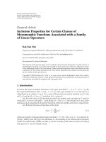
for every integer k ≥ 0. The partitioning is represented in the following diagram:
8
1.3. The Triangle Map

0

1


2

3

4
The triangle map
T :
∞

k=0

k
→ 
is then given by
T (x, y) =

y
x
,
1 − x − ky
x

if (x, y) ∈ 
k
.
To each (a, b) ∈  assign the sequence (a
1
, a
2

, ) if for every k > 0,
T
k
(a, b) ∈ 
a
k
.
If for some k it happens that T
k
(a, b) ∈ {(x, 0) : 0 ≤ x ≤ 1}, we stop the iterative process
and terminate the sequence. We call this sequence the triangle sequence associated with
(a, b).
We want to represent the triangle map using matrix notation. To do this, start by
defining a cone 
∗
such that

∗
= {(b
0
, b
1
, b
2
) : b
0
≥ b
1
≥ b
2

≥ 0},
and construct a projection map π : R
3
→ R
2
given by
π(b
0
, b
1
, b
2
) =

b
1
b
0
,
b
2
b
0

.
9
1.3. The Triangle Map
Then π(
∗
) = , our “base” triangle.

Now define the vectors
v
1
=


1
0
0


, v
2
=


1
1
0


, v
3
=


1
1
1



and note that π maps v
1
, v
2
, and v
3
to the vertices of .
This implies that
(v
1
, v
2
, v
3
) =


1 1 1
0 1 1
0 0 1


= B
is the R
3
representation of our base triangle ; operations on this matrix will facilitate the
desired partitioning.
To subdivide  in a way identical to the triangle map constructed above, we define
matrices

A
0
=


0 0 1
1 0 0
0 1 1


, A
1
=


1 0 1
0 1 0
0 0 1


and notice that
(v
1
, v
2
, v
3
)A
0
= (v

2
, v
3
, v
1
+ v
3
)
and
(v
1
, v
2
, v
3
)A
1
= (v
1
, v
2
, v
1
+ v
3
).
This implies that the action of A
0
and A
1

on B produces a disjoint partition of .
Now apply A
1
k times to B, and then apply A
0
once; in this process, ’s vertices are
sent to the vertices of

k
= {(x, y) ∈  : 1 − x − ky ≥ 0 > 1 − x − (k + 1)y}.
This allows us the define the triangle map as
T :
∞

k=0

k
→ 
where
T (x, y) = π

(1, x, y)

BA
−1
0
A
−k
1
B

−1

T

10
1.4. A Family of 216 Multidimensional Continued Fraction Algorithms: TRIP Maps
if (x, y) ∈ 
k
. Doing out the matrix multiplication, the above definition yields
T (x, y) =

y
x
,
1 − x − ky
x

,
which is identical to the map we defined above.
This enables us to assign the triangle sequence (a
1
, a
2
, ) to a point (a, b) ∈  by letting
a
i
equal k if T
i
(x, y) ∈ 
k

; again, if for any k we have T
k
(a, b) ∈ {(x, 0) : 0 ≤ x ≤ 1}, we
stop the iterative process and terminate the sequence. In order to see that periodicity in the
triangle sequence implies cubic irrationality, we consider the action of the map T : R
3
→ R
3
before we project the output into R
2
, defined by
T (1, x, y) = (1, x, y)

BA
−1
0
A
−k
1
B
−1

T
which reduces to
T (1, x, y) = (1, x, y)


0 0 1
1 0 −1
0 1 −k



.
If the original components of the point (x, y) ∈ , x and y, are both algebraic, each will
be algebraic of degree no more than 3 if we can find matrices B and A, where both B and
A can be written as products of matrices having the form


0 0 1
1 0 −1
0 1 −k


such that (1, x, y) is some eigenvector of the matrix AB
−1
; i.e.,
(1, x, y)AB
−1
= λ(1, x, y),
where λ is the associated eigenvalue. Of course, we require AB
−1
= I.
1.4 A Family of 216 Multidimensional Continued Frac-
tion Algorithms: TRIP Maps
Again, this section relies on material presented in [2] and [5].
11
1.4. A Family of 216 Multidimensional Continued Fraction Algorithms: TRIP Maps
Dasaratha, et. al [2] conjecture that there exists no unique, single multidimensional con-
tinued fraction algorithm capable of solving the Hermite problem. This conjecture motivates
looking at families of multidimensional continued fractions. In particular, the family of 216

TRIP maps (short for triangle partition maps) arises if, at each step of the division of the
base triangle  we allow for three permutations of the vertices of its R
3
representation.
To construct the other 215 TRIP maps, it is important to note that there was nothing
special about the ordering of the vertices (v
1
, v
2
, v
3
). Hence, we will allow permutations of
the initial vertices by some σ ∈ S
3
3
, by some τ
1
∈ S
3
3
after applying A
1
, and by some τ
0
∈ S
3
3
after applying A
0
.

This leads us to define the matrices
F
0
= σA
0
τ
0
, F
1
= σA
1
τ
1
for each (σ, τ
0
, τ
1
) ∈ S
3
3
.
In particular, we denote the permutation matrices as follows:
e =


1 0 0
0 1 0
0 0 1



,
(12) =


0 1 0
1 0 0
0 0 1


,
(13) =


0 0 1
0 1 0
1 0 0


,
(23) =


1 0 0
0 0 1
0 1 0


,
(123) =



0 1 0
0 0 1
1 0 0


,
(132) =


0 0 1
1 0 0
0 1 0


.
12
1.5. TRIP Sequences and TRIP Tree Sequences
The application of F
0
and F
1
to (the R
3
representation of) any triangle in (the R
3
representation of)  partitions it into two triangles. Hence, instead of using A
0
and A
1

, we
can subdivide  using F
0
and F
1
. Using these F
0
and F
1
, we can define 216 triangle partition
maps (TRIP maps, for short), each for one of the 216 permutation triplets in S
3
3
.
Let us make this definition more rigorous. Let 
k
be the triangle defined by the three
points obtained from applying the projection map π to the columns of the matrix BF
k
1
F
0
.
Then define a TRIP map as T
σ,τ
0
,τ
1
:


∞
k=0

k
→  where
T
σ,τ
0
,τ
1
(x, y) = π

(1, x, y)

BF
−1
0
F
−k
1
B
−1

T

if (x, y) ∈ 
k
. Of course, the original triangle map corresponds to T
e,e,e
.

We have calculated the explicit forms of T
σ,τ
0
,τ
1
(x, y) and T
−1
σ,τ
0
,τ
1
(x, y) for all (σ, τ
0
, τ
1
) ∈
S
3
3
; they are discussed in Chapters 2 and 3, and are explicitly presented in Appendices A
and B.
1.5 TRIP Sequences and TRIP Tree Sequences
This section relies on material presented in [2].
The above definition of T
σ,τ
0
,τ
1
(x, y) allows us to create the analogue of the triangle
sequence for all 216 TRIP maps: given (x, y) ∈ , let a

i
equal k if T
i
σ,τ
0
,τ
1
(x, y) ∈ 
k
. Then
the sequence (a
1
, a
2
, ) is the TRIP sequence induced by T
σ,τ
0
,τ
1
that is assigned to (x, y).
The sequence assigned to (a, b) ∈  terminates if there exists a k such that
T
k
(a, b) ∈ {(x, y) : (x, y) /∈
∞

i=0

i
}.

Of course, the triangle sequence is simply the TRIP sequence induced by T
e,e,e
that is assigned
to (x, y) ∈ .
It is important to note that there exists another related way of obtaining a sequence from
a point (x, y) ∈ . In particular, given (σ, τ
0
, τ
1
) ∈ S
3
3
, define the triangle
(i
1
, i
2
, i
n
) = BF
i
1
F
i
2
···F
i
n
.
13

1.6. Transfer Operators
Then, given (x, y) ∈ , define i
j
∈ {0, 1} such that (x, y) ∈ (i
1
, i
2
, . . . , i
j
, . . . , i
n
). The
sequence thus obtained, (i
1
, i
2
, . . . , i
n
), is the TRIP tree sequence induced by T
σ,τ
0
,τ
1
that is
assigned to (x, y).
It is easy to convert between the TRIP and TRIP tree sequences of a point (x, y) ∈ 
induced by a given T
σ,τ
0
,τ

1
: say the TRIP tree sequence is (1
a
1
, 0, 1
a
2
, 0, 1
a
3
, . . . ), where 1
a
i
stands for 1 appearing a
i
times consecutively. Then the corresponding TRIP sequence is
(a
1
, a
2
, a
3
, . . . ).
1.6 Transfer Operators
This section relies on material from [5].
Much work has been devoted to working out the statistics of the terms appearing in
the continued fraction representations of real numbers (see, for example, [9]). As per [5],
some important research inspired by this line of work (see [12]) relies on use of the transfer
operator
Lf(x) =

∞

n=1
1
(n + x)
2
f

1
n + x

;
under certain conditions on f(x), the largest eigenvalue of this transfer operator is 1, with
associated eigenfunction
h(x) =
1
1 + x
[12].
It is natural to inquire if there exist analogous results for multidimensional continued
fractions, and in particular for TRIP maps. First, we must develop the notion of a transfer
operator. Consider a dynamical system (X, S, µ, T ) (see Section 1.11 for the definition). A
transfer operator linearly maps functions defined on X in some vector space to functions
defined on X in some vector space. For a more concrete definition, choose a function g :
X → R. The transfer operator, call it L
T
, acting on f : X → R is given by
L
T
f(x) =


y:T(y)=x
g(y)f(y).
14
1.8. Polynomial- and Non-Polynomial-Growth TRIP Maps
If T is differentiable, we usually choose g =
1
|Jac(T )|
.
Extending this definition to the case of TRIP maps, we define our transfer operators to
be
L
T
σ,τ
0
,τ
1
f(x, y) =

(a,b):T
σ,τ
0
,τ
1
(a,b)=(x,y)
1
|Jac(T
σ,τ
0
,τ
1

(a, b))|
f(a, b).
As an example,
L
T
e,e,e
f(x, y) =
∞

k=0
1
(1 + kx + y)
3
f

1
1 + kx + y
,
x
1 + kx + y

.
We have calculated the explicit form of L
T
e,e,e
f(x, y) for all (σ, τ
0
, τ
1
) ∈ S

3
3
; these are
presented in Appendix E. A sample calculation of the explicit form of a transfer operator is
presented in Chapter 6.
1.7 Interlude
The Hermite problem was presented above to motivate the development of TRIP maps
by showing a potential application. Having placed TRIP maps in this context, thereby
establishing their importance in their own right, from now on we focus on the functional
analysis behind these TRIP maps, discussing their explicit form and ergodic properties – as
well as the form, spectrum, and nuclearity of the associated transfer operators.
1.8 Polynomial- and Non-Polynomial-Growth TRIP Maps
We see that the transfer operator corresponding to T
e,e,e
has a particularly nice form, in that
the denominator of the factor
1
(1+kx+y)
3
is (non-trivially) polynomial in k. In general, we will
be concerned with the form of the transfer operator L
T
σ,τ
0
,τ
1
where
L
T
σ,τ

0
,τ
1
f(x, y) =

(a,b):T
σ,τ
0
,τ
1
(a,b)=(x,y)
1
|Jac(T
σ,τ
0
,τ
1
(a, b))|
f(a, b)
If the denominator of
1
Jac(T
σ,τ
0
,τ
1
(a,b))
is (non-trivially) polynomial in k (also allowing for
factors of (−1)
k

) for a given T
σ,τ
0
,τ
1
, then that T
σ,τ
0
,τ
1
gives rise to a polynomial-growth
15
1.9. Combo TRIP Maps and Polynomial-Growth
transfer operator, and is itself polynomial-growth; otherwise, both L
T
σ,τ
0
,τ
1
and T
σ,τ
0
,τ
1
are
non-polynomial-growth.
By direct calculation of the explicit form of the transfer operators, presented in Ap-
pendix E, we have shown that exactly half of the 216 TRIP maps are polynomial-growth. In
addition, we identified the origin of polynomial-growth by showing that that a TRIP map
T

σ,τ
0
,τ
1
is polynomial-growth if and only if the eigenvalues of the associated F
1
= σA
1
τ
1
all
have magnitude 1; theorems regarding polynomial-growth in TRIP maps are presented in
Chapter 8. We use these results in Chapter 10 to classify patterns appearing in the visual
representations of the partitions

∞
k=0

k
induced on  by T
σ,τ
0
,τ
1
.
1.9 Combo TRIP Maps and Polynomial-Growth
We obtain a larger class of maps by allowing compositions of TRIP maps [2]. As an example,
we might perform the first division of  using the permutation triplet (σ, τ
0
, τ

1
), the next
using the permutation triplet (σ
2
, τ
02
, τ
12
), etc. We can represent such compositions as T
1
◦
T
2
. . . ◦ T
n
, where, of course, each subscript is short for a permutation triplet.
Further, we can consider a composition of TRIP maps T
1
◦T
2
◦ ◦T
i
, where {T
j
}, j ∈ λ,
with λ some indexing set such that λ ⊂ {1, 2, , i}, are polynomial-growth maps, and the
rest are non-polynomial-growth. In Chapter 9, we prove that the corresponding transfer
operator will be polynomial in all k
j
such that j ∈ λ, and exponential in all k

l
such that
l ∈ {1, 2, . . . , i} \ λ.
We have also identified the origin of polynomial-growth in such arbitrary finite composi-
tions of TRIP maps. Let M
1
=


BF
−1
0
F
−k
1
1
B
−1

T

−1
, M
2
=


BF
−1
0

F
−k
2
1
B
−1

T

−1
, and
so on until M
i
=


BF
−1
0
F
−k
i
1
B
−1

T

−1
. Then the composition T

1
◦T
2
◦ ◦T
i
is polynomial-
growth in k
j
, j ∈ {1, 2, . . . , i} if and only if the eigenvalues of F
1
j
all have magnitude 1. This
result is presented in Chapter 9.
16
1.11. Ergodic Theory
1.10 Nuclearity and Spectral Gaps for Transfer Oper-
ators Associated with Select TRIP Maps
In Chapters 11 and 12, we use analogues of the methods developed by Mayer, et. al in [12],
and applied to the original TRIP map in [4] (the “Banach space approach” and the “Hilbert
space approach”) to show that the transfer operators corresponding to many additional TRIP
maps are also nuclear of trace class zero or possess spectral gaps. In particular, we have used
the Banach space approach to show that several additional TRIP maps have spectral gaps.
We have also used the Hilbert space approach to show that all transfer operators for which
we have found corresponding eigenfunctions of eigenvalue 1 are nuclear of trace class zero.
The Banach space approach involves finding an appropriate Banach space V on which L
T
acts, showing that L
T
is a linear map from V to V, and showing that the largest eigenvalue
of L

T
is 1 and has multiplicity 1.
To get at the Hilbert space approach, we consider a transfer operator related to L
T
,
namely L
T,µ
, defined by the property that for any measurable set A ⊂ , and for any
function f ∈ L
1
(µ)

A
L
T,µ
f(x, y)dµ =

T
−1
A
f(x, y)dµ,
where µ is the measure defined by the eigenfunction of eigenvalue 1 of the corresponding
L
T
. The fact that L
T
and L
T,µ
can be related by a simple transformation shows that these
transfer operators have identical spectra. Hence, if we can show that L

T,µ
is nuclear of trace
class zero, analogous results immediately follow for L
T
[4]. In order to show L
T,µ
is nuclear
of trace class zero, we write it as a sum over special functions satisfying particular properties.
1.11 Ergodic Theory
This section serves as a very brief introduction to ergodic theory, exactly following the outline
provided in [7], which in turn uses [17] as a reference.
Consider a set X and a collection of subsets of X, S. S is said to be a σ-algebra if it
17
1.12. Ergodicity of TRIP Maps
satisfies the following three properties: 1. X ∈ S, 2. If A ∈ S, then A
c
∈ S, and 3. If
A
1
, A
2
, A
3
, ··· ∈ S, then ∪
∞
n=1
A
n
∈ S.
A measure on S is a function µ : S → [0, ∞) where we require that 1. µ(∅) = 0, and 2.

If A
1
, A
2
, A
3
, ··· ∈ S are pairwise disjoint, then µ (∪
∞
n=1
A
n
) =

∞
n=1
µ(A
n
).
A set A ∈ X is measurable if A ∈ S.
We refer to the triplet (X, S, µ) as a measure space; in our discussion of the ergodicity of
TRIP maps, we will focus on the measure space (, B, λ), where B stands for Borel σ-algebra
and λ stands for the Lebesgue measure.
To get into ergodic theory, we must consider transformations induced on a measure space.
So let (X, S, µ) be a measure space. The transformation T : X → X is measurable if it is
such that for every A ∈ S, we also have that T
−1
(A) ∈ S. We refer to (X, S, µ, T) as a
dynamical system. A measurable T is nonsingular if for all A ∈ S, µ(T
−1
(A)) = 0 if and

only if µ(T (A)) = 0.
Further, A ∈ X is strictly T-invariant if A = T
−1
(A). We are now at a point where
we can define ergodicity. Let T be a nonsingular transformation. T is ergodic if for every
measurable, strictly T −invariant A ∈ X, µ(A) = 0 or µ(A
c
) = 0.
1.12 Ergodicity of TRIP Maps
Messaoudi, et al. [14] have shown that the original triangle map T
e,e,e
is ergodic. Jensen
has extended these arguments to show that the maps T
e,23,e
, T
e,23,23
, T
e,132,23
and T
e,23,132
are
ergodic [7]. In Chapter 13 we show that 2 more TRIP maps are ergodic using the analogues
of arguments outlined by Jensen in [7].
In addition to these ergodicity results, in Chapter 14 we present results regarding con-
vergence for combo TRIP maps and show in Chapter 15 that no TRIP sequence induced by
24 TRIP maps corresponds to a unique point.
18
1.14. Computational Methodology
1.13 Gauss-Kuzmin Distributions for TRIP Sequences
The probability distribution for terms appearing in the standard continued fraction expansion

of a number x ∈ R is called the Gauss-Kuzmin distribution [8]. In Chapter 16, we derive
analogues of the Gauss-Kuzmin distribution for TRIP sequences induced by select TRIP
maps, relying on the fact that these maps have been shown to be ergodic.
1.14 Computational Methodology
Mathematica was used to perform almost all of the calculations in this thesis; a discus-
sion regarding the general research approach, as well as more details regarding the use of
Mathematica, are found in Chapter 17.
19
Chapter 2
Explicit Form of TRIP Maps
The explicit form of T
σ,τ
0
,τ
1
(x, y) has been calculated for all (σ, τ
0
, τ
1
) ∈ S
3
3
. These explicit
forms are presented in Appendix A. Several explicit forms had already been calculated in
[5] and [2], but here we present all 216 explicit forms.
2.1 Sample TRIP Map Calculation
We will go through a sample calculation of the from of T
e,23,e
(x, y).
By definition, for (x, y) ∈ ,

T
e,23,e
(x, y) = π((1, x, y)

BF
−1
0
F
−k
1
B
−1

T
).
Here,
F
0
= (e)A
0
(23) =


0 1 0
1 0 0
0 1 1


,
so that

F
−1
0
=


0 1 0
1 0 0
−1 0 1


;
further,
F
1
= (e)A
1
(e) =


1 0 1
0 1 0
0 0 1


,
so that
F
−1
1

=


1 0 −1
0 1 0
0 0 1


,
20
2.1. Sample TRIP Map Calculation
and
F
−k
1
=


1 0 −k
0 1 0
0 0 1


.
We also have that
B
−1
=



1 −1 0
0 1 −1
0 0 1


.
From this, it follows that
BF
−1
0
F
−k
1
B
−1
=


0 1 0
0 0 1
−1 1 k + 1


,
so that
(1, x, y)

BF
−1
0

F
−k
1
B
−1

T
= (x, y, (k + 1)y + x − 1),
and hence
T
e,23,e
(x, y) = π((1, x, y)

BF
−1
0
F
−k
1
B
−1

T
) =

y
x
,
(k + 1)y + x − 1
x


.
21
Chapter 3
Explicit Form of TRIP Map Inverses
The explicit form of T
−1
σ,τ
0
,τ
1
(x, y) has been calculated for all (σ, τ
0
, τ
1
) ∈ S
3
3
. These explicit
forms are presented in Appendix B. These were calculated from the definition
T
−1
σ,τ
0
,τ
1
(x, y) = π((1, x, y)


BF

−1
0
F
−k
1
B
−1

T

−1
).
The explicit form associated with T
e,e,e
had already been calculated in [5], but here we present
all 216 explicit forms.
3.1 Sample TRIP Map Inverse Calculation
We will go through a sample calculation of the from of T
−1
e,23,e
(x, y).
We have that
T
−1
e,23,e
(x, y) = π((1, x, y)


BF
−1

0
F
−k
1
B
−1

T

−1
).
From Chapter 2, we know that
BF
−1
0
F
−k
1
B
−1
=


0 1 0
0 0 1
−1 1 k + 1


,
so that



BF
−1
0
F
−k
1
B
−1

T

−1
=


1 1 0
k + 1 0 1
−1 0 0


,
and hence
π((1, x, y)


BF
−1
0

F
−k
1
B
−1

T

−1
) =

1
(k + 1)x − y + 1
,
x
(k + 1)x − y + 1

.
22