A primal dual active set method for non negativity constrained total variation deblurring problems
Bạn đang xem bản rút gọn của tài liệu. Xem và tải ngay bản đầy đủ của tài liệu tại đây (1.3 MB, 55 trang )
A PRIMAL-DUAL ACTIVE-SET METHOD FOR
NON-NEGATIVITY CONSTRAINED TOTAL VARIATION
DEBLURRING PROBLEMS
DILIP KRISHNAN
B. A. Sc. (Comp. Engg.)
A THESIS SUBMITTED FOR THE DEGREE OF
MASTER OF SCIENCE
DEPARTMENT OF MATHEMATICS
NATIONAL UNIVERSITY OF SINGAPORE
2007
Acknowledgements
The research work contained in this thesis would not be possible without the rigorous,
methodical and enthusiastic guidance of my supervisor, Dr. Andy Yip. Andy has opened
my eyes to a new level of sophistication in mathematical thinking and relentless questioning.
I am grateful to him for this. I would like to thank my co-supervisor, Dr. Lin Ping, for his
support and guidance over the last two years. Thanks are also due to Dr. Sun Defeng for
useful discussions on semi-smooth Newton’s methods. Last but not least, I would like to
thank my wife, Meghana, my parents, and brother for their love and support through the
research and thesis phases.
i
Contents
1 Introduction 1
1.1 Image Deblurring and Denoising . . . . . . . . . . . . . . . . . . . . . . . . 1
1.2 Total Variation Minimization Problems . . . . . . . . . . . . . . . . . . . . 2
2 The Non-Negatively Constrained Primal-Dual Program 8
2.1 Dual and Primal-Dual Approaches . . . . . . . . . . . . . . . . . . . . . . . 8
2.2 NNCGM Algorithm . . . . . . . . . . . . . . . . . . . . . . . . . . . . . . . 11
2.3 Preconditioners . . . . . . . . . . . . . . . . . . . . . . . . . . . . . . . . . . 14
2.4 Comparative Algorithms . . . . . . . . . . . . . . . . . . . . . . . . . . . . . 15
3 Numerical Results 18
3.1 Introduction . . . . . . . . . . . . . . . . . . . . . . . . . . . . . . . . . . . . 18
3.2 Numerical Comparison with the PN and AM Algorithms . . . . . . . . . . . 18
3.3 Robustness of NNCGM . . . . . . . . . . . . . . . . . . . . . . . . . . . . . 28
4 Conclusion 35
A Derivation of the Primal-Dual Program and the NNCGM Algorithm 41
A.1 The Primal-Dual Program . . . . . . . . . . . . . . . . . . . . . . . . . . . . 41
A.2 Optimality Conditions . . . . . . . . . . . . . . . . . . . . . . . . . . . . . . 42
A.3 The NNCGM Algorithm . . . . . . . . . . . . . . . . . . . . . . . . . . . . . 43
B Default Parameters for Given Data 49
ii
Summary
This thesis studies image deblurring problems using a total variation based model, with
a non-negativity constraint. The addition of the non-negativity constraint improves the
quality of the solutions but makes the process of solution a difficult one. The contribution
of our work is a fast and robust numerical algorithm to solve the non-negatively constrained
problem. To overcome the non-differentiability of the total variation norm, we formulate the
constrained deblurring problem as a primal-dual program which is a variant of the formu-
lation proposed by Chan, Golub and Mulet [1] (CGM) for unconstrained problems. Here,
dual refers to a combination of the Lagrangian and Fenchel duals. To solve the constrained
primal-dual program, we use a semi-smooth Newton’s method. We exploit the r elationship,
established in [2], between the se mi-smooth Newton’s method and the Primal-Dual Active
Set (PDAS) method to achieve considerable simplification of the computations. The main
advantages of our proposed scheme are: no parameters need significant adjustment, a stan-
dard inverse preconditioner works very well, quadratic rate of local convergence (theoretical
and numerical), numerical evidence of global convergence, and high accuracy of solving the
KKT system. The scheme shows robustness of performance over a wide range of parame-
ters. A comprehensive set of numerical comparisons are provided against other methods
to solve the same problem which show the speed and accuracy advantages of our scheme.
The Matlab and C (Mex) code for all the experiments conducted in this thesis may be
downloaded from />∼
mhyip/nncgm/.
iii
Chapter 1
Introduction
1.1 Image Deblurring and Denoising
In this thesis, we study models to solve image deblurring and denoising problems. During
the image acquisition process, images can suffer from various types of degradation. Two of
the most common problems are that of noise and blurring. Noise is introduced because of
the behaviour of the camera capture circuitry and exposure conditions. Blurring may be
introduced due to a combination of physical phenomena and camera processes. For example,
during the acquisition of satellite (atmospheric) images, the effect of the atmosphere acts
as a blurring filter to blur the captured images of heavenly b odies.
Image blur is usually modelled as a convolution of the image data with a blurring kernel.
The kernel may vary depending on the type of blur. Two common blurs are Gaussian blur
and out-of-focus blur. Image noise is usually modelled as additive Gaussian distributed
noise or uniformly distributed noise. Denoising can be considered to be a special case of
deblurring with identity blur.
Digital images are represented as two-dimensional arrays f(x, y). where each integer
coordinate (x, y) represents a single pixel. At each pixel, an integer value which varies
between 0 and 255, for images of bit depth 8, represents the intensity or gray level of the
pixel. 0 represents the color black, 255 represents the color white. All gray levels lie in
between these two exteme values. Image deblurring may be represented as f = k ∗ u + n,
where f is the observed degraded image, u is the original image, k is the blurring function
1
2
and n is the additive noise.
Deblurring and denoising of images is important for scientific and aesthetic reasons. For
example, police agencies require deblurring of images captured from security cameras; de-
noising of images helps significantly in their compression; deblurring of atmospheric images
is useful for the accurate identification of the heavenly bodies. See [3], [4] for more examples
and overview.
A number of different models have been proposed to solve deblurring and denoising
problems. It is not our purpose here to study all the different models. We restrict our
attention to a model based on the Total Variation, which has proven to be succesful in
solving a number of different image processing problems, including deblurring and denoising.
1.2 Total Variation Minimization Problems
Total Variation (TV) minimization problems were first introduced into the context of image
denoising in the seminal paper [5] by Rudin, Osher and Fatemi. They have proven to be
successful in dealing with image denoising and deblurring problems [1,6–8], image inpainting
problems [9], and image decomposition [10]. Recently, they have also been applied in various
areas such as CT imaging [11,12] and confocal microscopy [13]. The main advantage of the
TV formulation is the ability to preserve edges in the image. This is due to the piecewise
smooth regularization property of the TV norm.
A discrete version of the unconstrained TV deblurring problem proposed by Rudin et al.
in [5] is given by
min
u
1
2
Ku − f
2
+ βu
T V
, (1.1)
where · is the l
2
norm, f is the observed (blurred and noisy) data, K is the blurring
operator corresponding to a point spread function (PSF), u is the unknown data to be
recovered, and ·
T V
is the discrete TV regularization term. We assume that the m ×
n images u = (u
i,j
) and f = (f
i,j
) have been rearranged into a vector form using the
lexicographical ordering. Thus, K is an mn × mn matrix. The discrete TV norm is defined
3
as
u
T V
:=
m−1
i=1
n−1
j=1
|(∇u)
ij
|, where (∇u)
ij
=
u
i+1,j
− u
i,j
u
i,j+1
− u
i,j
. (1.2)
Here, i and j refer to the pixel indices in the image and | · | is the Euclidean norm for R
2
.
Regularization is necessary due to the presence of noise, see [14]. Without regularization,
noise amplification would be so severe that the resulting output data is useless, especially
when K is very ill-conditioned. Even when K is well-conditioned, regularization is still
needed to remove noise. The regularization parameter β needs to be selected as a tradeoff
between oversmoothing and noise amplification. When K = I, the deblurring problem
becomes a pure denoising problem. When K is derived from a non-trivial PSF (i.e. apart
from the Dirac Delta function), the problem is harder to solve since the pixels of f are
coupled together to a greater degree. When K is unknown, the problem becomes a blind
deblurring problem [6,15]. In this paper, we assume that the PSF, and hence K, is known.
One of the major reasons for ongoing research into TV deblurring problems is that
the non-differentiability of the TV norm makes it a difficult task to find a fast numerical
method. The (formal) first order derivative of the TV norm involves the term
∇u
|∇u|
which
is degenerate when |∇u| = 0. This could happen in flat areas of the image. Methods that
can effectively deal with such singularities are still actively sought.
A number of numerical methods have been proposed for unconstrained TV denoising
and/or deblurring models. These include partial differential equation based methods such as
explicit [5], semi-implicit [16] or operator splitting schemes [17] and fixed point iterations [7].
Optimization oriented techniques include Newton-like methods [1], [18], [8], multilevel [19],
second order cone programming [20] and interior-point methods [21]. Recently, graph based
approaches have also been studied [22]. It is also possible to apply Additive Operator
Splitting (AOS) based schemes such as those proposed originally in [23] to solve in a fast
manner, the Euler-Lagrange equation corresponding to the primal problem.
Carter [24] presents a dual formulation of the TV denoising problem and studies some
primal-dual interior-point and primal-dual relaxation methods. Chambolle [25] presents a
semi-implicit scheme and Ng et al. [26] present a semi-smooth Newton’s method for solving
the same dual problem. These algorithms have the advantage of not requiring an extra
4
regularization of the TV norm. Being faithful to the original TV norm without applying
any regularization, these methods often require many iterations to converge to a moderate
level of accuracy for the underlying optimization problem is not strictly convex.
Hinterm¨uller and Kunisch [27] have derived a dual version of an
anisotropic TV deblurring problem. In the anisotropic formulation, the TV norm u
T V
in
Eq. (1.2) is replaced with
i,j
|(∇u)
ij
|
1
where | · |
1
is the l
1
norm for R
2
. This makes the dual
problem a quadratic one with linear bilateral constraints. In contrast, the isotropic formu-
lation is based on the l
2
norm and has the advantage of being rotation invariant. However,
the dual problem corresponding to the isotropic TV norm has quadratic constraints which
are harder to deal with. Hinterm¨uller and Kunisch have solved the anisotropic formula-
tion using a primal-dual active-set method, but the algorithm requires several additional
regularization terms.
Chan, Golub and Mulet present a primal-dual numerical method [1]. This algorithm
(which we henceforth call the CGM algorithm) simultaneously solves both the primal and
(Fenchel) dual problems. In this work, we propose a variant of their algorithm to handle
the non-negativity constraint.
It should be noted that many of the aforementioned numerical methods are specific to
denoising and cannot be readily extended to a general deblurring problem. Fewer papers
focus on TV deblurring problems. Still fewer focus on constrained TV deblurring prob-
lems. But our method works for the more difficult non-negativity constrained isotropic TV
deblurring problem and is faster than other existing methods for solving the same problem.
Image values which represent physical quantities such as photon count or energies are
often non-negative. For example, in applications such as gamma ray spectral analysis [28],
astronomical imaging and spectroscopy [29], the physical characteristics of the problem
require the recovered data to be non-negative. An intuitive approach to ensuring non-
negativity is to solve the unconstrained problem first, followed by setting the negative
components of the resulting output to zero. However, this approach may result in the
presence of spurious ripples in the reconstructed image. Chopping off the negative values
may also introduce patches of black color which could be visually unpleasant. In biomedical
imaging, the authors in [12, 13] also stressed the importance of non-negativity in their TV
5
based models. But they obtain non-negative results by tuning a regularization parameter
similar to the β in Eq. (1.1). This may cause the results to be under- or over-regularized.
Moreover, there is no guarantee that such a choice of the parameter exists. Therefore, a
non-negativity constraint on the deblurring problem is a natural requirement.
The non-negatively constrained TV deblurring problem is given by
min
u,u≥0
1
2
Ku − f
2
+ βu
T V
. (1.3)
This problem is convex for all K and is strictly convex when K is of full rank. We shall
assume that K is of full rank so that the problem has a unique solution. For denoising
problems, imposing the non-negativity constraint becomes unnecessary for it is equivalent
to solving the unconstrained problem followed by setting the negative components to zero.
For deblurring problems, even if the observed data are all positive, the deblurred result may
contain negative values if non-negativity is not enforced.
Schafer et al. [28], have studied the non-negativity constraint on gamma-ray spectral
data and synthetic data. They have demonstrated that such a constraint helps not only
in the interpretability of the results, but also helps in the reconstruction of high-frequency
information beyond the Nyquist frequency (in case of bandlimited signals). Reconstruction
of the high-frequency information is an important requirement for image processing since
the details of the image are usually the edges.
Fig. 1.1 gives another example. The reconstructions 1.1(d) and 1.1(e) based on the
unconstrained primal-dual method presented in [1] show a larger number of spurious spikes.
It is also clear that the intuitive method of solving the unconstrained problem and setting
the negative components to zero still causes a number of spurious ripples. In contrast, the
constrained solution 1.1(c) has much fewer spurious ripples in the recovered background.
The unconstrained results have larger l
2
reconstruction error compared to the constrained
reconstruction.
Some examples showing the increased reconstruction quality of imposing non-negativity
can be found in [30]. Studies on other non-negativity constrained deblurring problems
such as Poisson noise model, linear regularization and entropy-type penalty can be found
in [31,32].
6
20
40
60
20
40
60
−100
0
100
200
Original
(a)
20
40
60
20
40
60
−100
0
100
200
Noisy and Blurred
(b)
20
40
60
20
40
60
−100
0
100
200
NNCGM
(c)
20
40
60
20
40
60
−100
0
100
200
CGM
(d)
20
40
60
20
40
60
−100
0
100
200
CGM (Neg components set to 0)
(e)
Figure 1.1: Comparison of constrained and unconstrained deblurring. (a) Original syn-
thetic data. (b) Blurred and noisy data with negative components. (c) Non-negatively
constrained NNCGM result; l
2
error = 361.43. (d) Unconstrained CGM result; l
2
error =
462.74. (e) Same as (d) but with negative components set to 0; l
2
error = 429.32.
7
Very few numerical approaches have been studied for non-negatively constrained total
variation deblurring problems. In [30, 33], a projected Newton’s method based on the
algorithm of [34] is presented to solve the non-negatively constrained problem. We study
the performance of this algorithm in this work. Fu et al. [21] present an algorithm based
on interior-point methods, along with very effective preconditioners. The total number of
outer iterations is small. However, the inner iterations, corresponding to Newton steps in the
interior-point method, take long to converge. Moreover, Fu et al. study the anisotropic TV
formulation, which can be reduced to a linear programming problem, whereas the isotropic
formulation is more difficult to solve. We have studied the interior-point method for the
isotropic TV norm and observed significant slow down in the inner iterations as the outer
iterations proceed. This is because of the increased ill-conditioning of the linear systems
that are to be solved in the inner iterations. In contrast, the primal-dual method presented
in this work does not suffer from this drawback – the number of inner conjugate gradient
(CG) iterations [35] shows no significant increase as the system approaches convergence.
The rest of the thesis is organized as follows: Chapter 2 presents our proposed primal-
dual method (which we call NNCGM) for non-negatively constrained TV deblurring, along
with two other algorithms to which we compare the performance of the NNCGM algorithm.
These two algorithms are a dual-only Alternating Minimization method and a primal-only
Projected Newton’s method. Chapter 3 provides numerical results to compare NNCGM
with these two methods and also shows the robustness of NNCGM. Chapter 4 gives conclu-
sions. Appendix A gives the technical details of the derivation of the primal-dual formulation
and the NNCGM algorithm. Appendix B gives the default parameters that were used for
all the numerical results given in this thesis.
A paper [36] based on the results presented in this thesis has recently (August 2007)
been accepted for publication in the IEEE Transactions on Image Processing.
Chapter 2
The Non-Negatively Constrained
Primal-Dual Program
2.1 Dual and Primal-Dual Approaches
Solving the primal TV deblurring problem, whether unconstrained or constrained, poses
numerical difficulties due to the non-differentiability of the TV norm. This difficulty is
usually overcome by the addition of a perturbation . That is, to replace |∇u| with |∇u|
=
|∇u|
2
+ which is a differentiable function. The trade-off in choosing this smoothing
parameter is the reconstruction error versus the speed of convergence. The smaller the
perturbation term, the more accurate is the final reconstruction. However, convergence
takes longer since the corresponding objective function to b e optimized becomes increasingly
closer to the original non-differentiable objective function. See [37] for more details on
convergence in relation to the value of .
Owing to the above numerical difficulties, some researchers have studied a dual approach
to the TV deblurring problem. Carter [24] and Chambolle [25] present a dual problem based
on the Fenchel dual formulation for the TV denoising problem. See [38] for details on the
Fenchel dual. Chambolle’s scheme is based on the minimization problem
min
p,|p
i,j
|≤1
f + βdivp
2
. (2.1)
8
9
Here,
p
i,j
=
p
x
i,j
p
y
i,j
(2.2)
is the dual variable at each pixel l ocation with homogeneous Dirichlet boundary conditions
p
x
0,j
= p
x
m,j
= 0 for all j and p
y
i,0
= p
y
i,n
= 0 for all i. The vector p is a concatenation of all
p
i,j
. The discrete divergence operator div is defined such that the vector divp is given by
(divp)
i,j
= p
x
i,j
− p
x
i−1,j
+ p
y
i,j
− p
y
i,j−1
. (2.3)
It can be shown (see [25]) that (−div)
T
= ∇ defined in (1.2). The constraints |p
i,j
| ≤ 1 are
quadratic after squaring both sides. The update is given by
p
n+1
i,j
=
p
n
i,j
+ τβ(∇(βdivp + g))
i,j
1 + τβ|(∇(βdivp + g))
i,j
|
, ∀ i, j,
where τ is the step size (which, as shown in [25], needs to be less than 1/8). Once the
optimal solution, denoted by p
∗
, is obtained, the denoised image u
∗
can be reconstructed
by u
∗
= βdivp
∗
+ f. An interesting aspect of the algorithm is that even without the -
perturbation of the TV norm, the objective function becomes a quadratic function which is
infinitely differentiable. But the dual variable p becomes constrained. Unfortunately, being
based on a steepest descent technique, the algorithm slows down towards convergence and
requires a large number of iterations for even a moderate accuracy.
Hinterm¨uller and Kunisch [27] have also used the Fenchel dual approach to formulate a
constrained quadratic dual problem and to derive a very effective method. They consider
the case of anisotropic TV norm so that the dual variable is bilaterally constrained, i.e.
−1 ≤ p
i,j
≤ 1, whereas the constraints in Eq. (2.1) are quadratic. The smooth (quadratic)
nature of the dual problem makes it much more amenable to solution by a Newton-like
method. To deal with the bilateral constraints on p, the authors propose to use the Primal-
Dual Active-Set (PDAS) algorithm. Consider the general quadratic problem
min
y≤ψ
1
2
y, Ay − f, y
whose KKT system [39] is given by
Ay + λ = f,
C(y, λ) = 0,
10
where C(y, λ) = λ − max(0, λ + c(y − ψ)) for an arbitrary positive constant c, and λ is the
Lagrange multiplier. The max operation is understood to be component-wise. Then the
PDAS algorithm is given by
1. Initialize y
0
, λ
0
. Set k = 0.
2. Set I
k
= {i : λ
k
i
+ c(y
k
− ψ)
i
≤ 0} and A
k
= {i : λ
k
i
+ c(y
k
− ψ)
i
> 0}.
3. Solve
Ay
k+1
+ λ
k+1
= f,
y
k+1
= ψ on A
k
,
λ
k+1
= 0 on I
k
.
4. Stop, or set k = k + 1 and return to Step 2).
In their work in [2], the authors show that the PDAS algorithm is equivalent to a semi-
smooth Newton’s method for a class of optimization problems that includes the dual
anisotropic TV deblurring problem. Local superlinear convergence results are derived.
Conditional global convergence results based on the properties of the matrix K are also
derived. However, their formulation only works for the anisotropic TV norm and the dual
problem requires several extra regularization terms to achieve a numerical solution.
Chan et al. [1] present a primal-dual numerical method which has a much better global
convergence behaviour than a primal-only method for the unconstrained problem. As the
name suggests, this algorithm simultaneously solves both the primal and dual problems.
The algorithm is derived as a Newton step for the following equations
p|∇u|
− ∇u = 0,
−βdivp − K
T
f + Au = 0,
where A := K
T
K + αI. At each Newton step, both the primal variable u and the dual
variable p are updated. The dual variable can be thought of as helping to overcome the
singularity in term div
∇u
|∇u|
. An advantage of this method is that a line search is required
only for the dual variable p to maintain the feasibility |p
i,j
| ≤ 1 whereas a line search for u
11
is unnecessary. Furthermore, while still requiring an -regularization as above, it converges
fast even when the perturbation is small. Our algori thm is inspired by the CGM method.
But the CGM method does not handle the non-negativity constraint on u.
Note that dual-only methods for TV deblurring need an extra l
2
regularization which is
a disadvantage for these methods. This is because the matrix (K
T
K)
−1
is involved and one
needs to replace it by (K
T
K + αI)
−1
to make it well-conditioned. In denoising problems,
we have K = I so that the ill-conditioning problem of (K
T
K)
−1
in dual methods is absent.
But in deblurring problems, some extra care needs to be taken. The modified TV deblurring
problem is then given by
min
u,u≥0
1
2
Ku − f
2
+ βu
T V
+
α
2
u
2
. (2.4)
Primal-dual methods such as CGM and our NNCGM do not require the extra l
2
regular-
ization term, i.e. α = 0. This is because K
T
K instead of (K
T
K)
−1
is involved in the
primal-dual formulation. See Appendix A.
2.2 NNCGM Algorithm
As stated above, our algorithm is inspired by the CGM method. Hence we call it the
NNCGM algorithm (Non-Negatively constrained Chan-Golub-Mulet). We derived the dual
of the constrained problem (2.4) as follows:
min
p,|p
i,j
|≤1
min
λ,λ≥0
1
2
B
1/2
(K
T
f + βdivp + λ)
2
, (2.5)
where B := (K
T
K+αI)
−1
. The dual variable p has constraints on it arising from the Fenchel
transform of the TV norm in the primal objective function Eq. (2.4). The variable λ has
a non-negativity constraint since it arises as a Lagrange multiplier for the non-negativity
constraint on u. See Appendix A for the detailed derivation. We remark that the parameter
α can be set to 0 in our method, see Chapter 2.1.
The primal-dual program associated with the problem (2.5) is given by:
p|∇u|
− ∇u = 0, (2.6)
−βdivp − K
T
f − λ + Au = 0, (2.7)
λ − max{0, λ − cu} = 0, (2.8)
12
where c is an arbitrary positive constant. We have identified the Lagrange multiplier for
λ ≥ 0 with the primal variable u. This leads to the presence of u in the system. Note that
we have transformed all inequality constraints and complementarity conditions on u and λ
into the single equality constraint in Eq. (2.8).
The NNCGM algorithm is essentially a se mi-smooth Newton’s method for the system
in Eq. (2.6)-(2.8). It has been shown by Hinterm¨uller et al. [27] that the semi-smooth
Newton’s method is equivalent to the PDAS algorithm for a certain class of optimization
problems. Although the equivalency does not hold in our problem, the two methods are
still highly related. We exploit this relationship, and use some ideas of the PDAS algorithm
to significantly simplify the computations involved in solving Eq. (2.6)-(2.8), see Appendix
A. The full NNCGM algorithm is as follows:
1. Select parameters based on Table B.1.
2. Initialize p
0
, u
0
, λ
0
. Set k = 0.
3. Set I
k
= {i : λ
k
i
− cu
k
i
≤ 0} and A
k
= {i : λ
k
i
− cu
k
i
> 0}. In the rest of the algorithm
below, these two quantities are represented as I and A respectively.
4. Compute δu
k
I
by solving the linear system using PCG (cf. Eq. (A.21)):
D
I
−βdiv
1
|∇u
k
|
I −
p
k
(∇u
k
)
T
+ (∇u
k
)(p
k
)
T
2|∇u
k
|
∇ + A
D
T
I
δu
k
I
= g(p
k
, u
k
, λ
k
). (2.9)
The details on the preconditioner used are given in Section 2.3.
5. Compute δp
k
by (cf. Eq. (A.19)):
δp
k
=
1
|∇u
k
|
×
I −
p
k
(∇u
k
)
T
|∇u
k
|
∇(D
T
I
δu
k
I
− D
T
A
u
k
A
) − F
1
(p
k
, u
k
, λ
k
)
.
6. Compute δλ
k
A
by (cf. Eq. (A.18)):
δλ
k
A
= −βD
A
divδp
k
+ A
AI
δu
k
I
+ D
A
F
2
(p
k
, u
k
, λ
k
) − A
A
u
k
A
.
7. Compute the step size s by s = ρ sup
γ
{|p
k
i,j
+ γδp
k
i,j
| ≤ 1 ∀ i, j}.
13
8. Update
p
k+1
= p
k
+ sδp
k
,
u
k+1
I
= u
k
I
+ δu
k
I
,
u
k+1
A
= 0,
λ
k+1
I
= 0,
λ
k+1
A
= λ
k
A
+ δλ
k
A
.
9. Either stop if the desired KKT residual accuracy is reached, or set k = k + 1 and
go back to Step 3). The KKT residual is given by
F
1
2
+ F
2
2
+ F
3
2
1/2
where
F
1
, F
2
, F
3
are defined by the left hand side of Eq. (2.6)-(2.8).
At every iteration, the current iterates for λ and u are used to predict the active (A
k
)
and inactive (I
k
) sets for the next iteration. This is the fundamental mechanism of the
PDAS method as presented in [2]. A line search is only required in Step 7), for p. We found
numerically that there was no need to have a line search in the u and λ variables. Occasional
infeasibility (i.e. violation of non-negativity) of these variables during the iterations did not
prevent convergence. The algorithm requires the specification of the following parameters:
1. c: c is a positive value used to determine the active and inactive sets at every iteration,
see Step 3) above. In our tests we found that the performance of the algorithm is
independent of the value of c, as long as c is a positive value. This is consistent with
the results obtained in [2]. Hence using a fixed value of c was sufficient for all our
numerical tests.
2. ρ: Setting ρ to 0.99 worked for all our numerical tests. This parameter is used only
to make the step size a little conservative.
3. : The perturbation constant is to be selected at a reasonably small value to achieve
a trade-off between reconstruction error and time for convergence. We found that
setting this to 10
−2
worked for all cases. Reducing it further did not significantly
reduce the reconstruction error. See Chapter 3 for results.
14
The regularization parameter β deci des the trade-off between the reconstruction error and
noise amplification. It is a part of the deblurring model, rather than our algorithm. The
value of β must be selected carefully for any TV deblurring algorithm.
Our NNCGM algorithm was inspired by using the CGM algorithm [1] to handle the TV
deblurring, and the PDAS algorithm [2] to handle the non-negativity constraint. The CGM
algorithm was shown to be very fast in solving the unconstrained TV deblurring problem,
and involved a minimal number of parameters. It also handles the inequality constraint on
the dual variable p by a simple line search. Furthermore, the numerical results i n [1] show a
locally quadratic rate of convergence. The PDAS algorithm handles unilateral constraints
effectively. While Hinterm¨uller and Kunisch [27] apply PDAS to handle the constraints
−1 ≤ p ≤ 1, we apply it to handle the non-negativity constraints u, λ ≥ 0. Under our
formulation, the quadratic constraints |p
i,j
| ≤ 1 for all i, j are implied Eq. (2.6). But we
found it more convenient to maintain the feasibility of these quadratic constraints by a
line search as in the CGM method. This can make sure that the linear system Eq. (2.9)
to solve in each Newton step is positive definite. Since the NNCGM method is basically
a semi-smooth Newton’s method and the system of equations to solve in our formulation
is strongly semi-smooth, it can therefore be expected that the NNCGM algorithm should
exhibit a quadratic rate of local convergence. The numerical results of Chapter 3 show a
locally quadratic rate of convergence.
2.3 Preconditioners
The most computationally intensive step of the NNCGM algorithm is Step 4) which involves
solving the linear system in Eq. (2.9). Though significantly smaller than the original
linear system (A.17) obtained by linearizing Eq. (2.6)-(2.8), it is still a large system.
We therefore explored the use of preconditioners, and discovered that the standard ILU
preconditioner [35] and the Factorized Banded Inverse Preconditioner (FBIP) [40] worked
well to speed up the solution of the linear system. The FBIP preconditioner, in particular,
worked extremely well. Using the FBIP preconditioner to solve the linear system requires
essentially O(N log N ) operations, where N is the total number of pixels in the image. This
15
is including the use of FFT’s for computations involving the matrix K.
The original system Eq. (A.17) has different characteristics in each of its blocks. It is
therefore harder to construct an effective preconditioner. In contrast, the reduced system
Eq. (2.9) has a simpler structure so that standard preconditioners work well.
2.4 Comparative Algorithms
We compare the performance of the NNCGM with two other algorithms: a primal-only
Projected Newton’s (PN) algorithm, and a dual-only Alternating Minimization (AM) algo-
rithm. To the best of our knowledge, the PN algori thm is the only algorithm proposed for
solving non-negativity constrained isotropic TV deblurring problems that is designed for
speed. The AM algorithm, derived by us, is a straightforward and natural way to reduce
the problem into subproblems that are solvable by existing solvers. A common way used
in application-oriented literature is to cast the TV minimization problem as a maximum
a posteriori estimation problem and then apply the expectation maximization (EM) algo-
rithm with multiplicative updates to ensure non-negativity [41]. The algorithm is usually
straightforward to implement. However, it is well-known that the convergence of EM-type
algorithms is slow. We experimented with a numb er of other algorithms as well, but the
performance of those algorithms was quite poor. For example, we tried using a barrier
method to maintain feasibility, but the method was very slow. The method given in Fu
et al .’s paper, [21] uses linear programming. Since they use the anisotropic model for the
TV, it is not a problem to maintain feasibility in their approach. We tri ed to adopt this
approach for our isotropic formulation, but it is difficult to maintain the feasibility of the
problem. Other interior-point methods require a feasible initial point, which is very difficult
to obtain for this problem owing to the non-linearity.
The PN algorithm is based on that presented in [30, 33]. At each outer iteration, active
and inactive sets are identified based on the primal variable u. Then a Newton step is taken
for the inactive variables whereas a projected steepest descent is taken for the active ones.
A line search ensures that the step size taken in the i nactive variables is such that they do
not violate the non-negativity constraint. A few parameters have to be modified to tune
16
the line search. The method is quite slow, for only a few inactive variables are updated at
each step. Active variables which are already at the boundary of the feasible set, cannot
be updated. Theoretically, once all the active variables are identified, the convergence is
quadratic. However, it takes many iterations to find all the active variables. In all of
our exp e riments, a quadratic convergence has not been observed within the limit of 300
iterations. More importantly, the Newton iterations diverge for many initial data since the
non-differentiability of the TV norm has not been dealt with properly [37].
A natural way to solve the dual problem (2.5) is by alternating minimization. The
AM algorithm is based on the convexity of the dual problem. The problem is solved by the
alternating solution of two subproblems: the λ subproblem for fixed p and the p subproblem
for a fixed λ. The λ subproblem is given by
min
λ,λ≥0
1
2
B
1/2
(b + λ)
2
, (2.10)
where
b = K
T
f + βdivp
c
,
and p
c
is the latest value of p from the previous iteration. The p subproblem is given by
min
p,|p
i,j
|≤1
1
2
B
1/2
(g + βdivp)
2
, (2.11)
where
g = K
T
f + λ
c
,
and λ
c
is the latest value of λ from the previous iteration. The solution of the λ subproblem
(2.10) uses the PDAS algorithm presented in [2]. The solution of the p subproblem (2.11) is
based on an extension of Chambolle’s steepest descent technique presented in [25], modified
for deblurring problems. The Euler-Lagrange equation corresponding to the problem is
−β [∇(B(βdivp + g))]
i,j
+ µ
i,j
p
i,j
= 0, ∀ i, j
where, as before, i, j refer to individual pixels in the image. Note that, as discussed earlier,
α > 0 in case of AM since this is a dual-only method. The above equation is used to derive
the following steepest-descent algorithm to solve the p subproblem:
p
n+1
i,j
=
p
n
i,j
+ τβ [∇(B(βdivp + g))]
i,j
1 + τβ| [∇(B(βdivp + g))]
i,j
|
, ∀ i, j.
17
Here, the step size τ is inversely proportional to the square root of the condition number of
K
T
K + αI which is very small for most reasonable choice of α (which is set to 0.008 in our
experiments). Thus, a large number of steps is expected. Once the dual problem is solved,
the solution u
∗
to the original problem is recovered as
u
∗
= B(K
T
f + βdivp
∗
+ λ
∗
),
where p
∗
and λ
∗
are the optimal solution to the dual problem. Duality arguments can be
used to show that the recovered optimal u
∗
satisfies the non-negativity constraint, cf. Eq.
(A.9) and (A.12).
Chapter 3
Numerical Results
3.1 Introduction
In this section, we present extensive numerical results to demonstrate the performance of
the NNCGM algorithm. We consider various conditions: different signal-to-noise ratios
(SNR), different types and sizes of point spread functions (PSF) and different values of
the smoothing parameter . We also show the robustness of the NNCGM algorithm with
respect to various parameters, and the performance of the FBIP preconditioner. The two
images that will be used for the comparison purposes are the License Plate and Satellite
images. The original images and typical results of TV deblurring for NNCGM are shown
in Fig. 3.1 and 3.2.
3.2 Numerical Comparison with the PN and AM Algorithms
In the tests below, we vary one condition at a time, leaving the others to their moderately
chosen values. In each test, we run each algorithm for a few different values of β and choose
the optimal β that minimizes the l
2
reconstruction error. Unless otherwise mentioned, all
results for NNCGM are with the use of the FBIP preconditioner, which significantly speeds
up the processing. For PN, we tested both the ILU and FBIP preconditioners, and they
caused the processing to be slower. Therefore, the results reported are without the use of
any preconditioner. Our primary interest in Fig. 3.3 to Fig. 3.10 is the outer iterations
18
19
20 40 60 80 100 120
20
40
60
80
100
120
(a)
20 40 60 80 100 120
20
40
60
80
100
120
(b)
20 40 60 80 100 120
20
40
60
80
100
120
(c)
Figure 3. 1: (a) Original License Plate image (128 × 128); (b) Blurred with Gaussian P SF
7 × 7, SNR 30dB; (c) TV deblurring results with NNCGM, β = 0.4.
20
20 40 60 80 100 120
20
40
60
80
100
120
(a)
20 40 60 80 100 120
20
40
60
80
100
120
(b)
20 40 60 80 100 120
20
40
60
80
100
120
(c)
20 40 60 80 100 120
20
40
60
80
100
120
(d)
20 40 60 80 100 120
20
40
60
80
100
120
(e)
20 40 60 80 100 120
20
40
60
80
100
120
(f)
Figure 3.2: Comparison of constrained and unconstrained deblurring. (a) Original Satellite
image (128 × 128); (b) Blurred and noisy data, Gaussian PSF of size 5 × 5, noise of SNR
15dB; (c) Non-negatively constrained deblurring result with β = 0.4, PSNR = 27.61dB;
(d) Unconstrained CGM with β = 0.4 and with negative components set to 0, PSNR =
25.96dB; (e) Contour plot of the result in (c); (f) Contour plot of the result in (d).
21
which are largely independent of the inner iterations.
Fig. 3.3 and 3.4 compare the convergence of NNCGM, PN and AM for different SNRs
of −10dB, 20dB, 50dB corresponding to high, medium and low level of noise respectively.
A fixed Gaussian PSF of size 9 × 9 and a fixed of 10
−2
were used. It is seen that the
NNCGM method reaches a very high accuracy of KKT residual of the order of 10
−6
and the
convergence is quadratic eventually. An even higher accuracy can be achieved with only a
few more iterations. The PN and AM methods become very slow in their progression after
about 50 iterations. The total number of outer iterations for the NNCGM method stays
below 70 even for a high noise level of −10dB.
Fig. 3.5 and 3.6 compare the convergence of NNCGM, PN and AM for varying Gaussian
PSF size with a fixed SNR of 20 dB and a fixed of 10
−2
.
Fig. 3.7 and 3.8 compare the convergence of NNCGM, PN and AM for varying with
fixed SNR of 20 dB and Gaussian PSF of size 9 × 9.
Fig. 3.9 and 3.10 compare the convergence of NNCGM, PN and AM for Gaussian blur
and out-of-focus blur with a fixed SNR of 20dB, a fixed PSF size of 9 × 9 and a fixed of
10
−2
, for the License Plate and Satellite images resp e ctively.
Tables 3.1 - 3.4 show the CPU timings in seconds and the peak signal-to-noise ratio
(PSNR) in dB for the plots from Fig. 3.3-3.10. The PSNR, defined by
10 log
10
255
2
1
mn
original − reconstructed
2
,
is a measure of image reconstruction error. Here, m × n are dimensions of the image. The
larger the PSNR, the smaller the error will be. The figures in parentheses after each CPU
timing for NNCGM refers to the total number of outer iterations required for each method.
In all cases, we set the maximum number of iterations to 300, for both the PN and AM
algorithms essentially stagnate after 300 iterations. The first sub-row in each row are License
Plate data and the second sub-row are Satellite data. In each case, bold letters highlight
the lowest CPU timings and the lowest reconstruction error (highest PSNR) among the
three algorithms. All the algorithms were implemented in Matlab 7.2. CPU timings were
measured on a Pentium D 3.2GHz processor with 4GB of RAM.
In most cases, the PN algorithm iterated for the maximum 300 iterations but did not