An indicator of the impact of climate change on north american bird populations

•
•
•

1

An Indicator of the Impact of Climate
Change on North American Bird
Populations
Jamie Alison
Thesis for MSc by Research
Supervised by Dr. Stephen Willis and Dr. Phil Stephens
Department of Biological and Biomedical Sciences
Durham University
2013
Abstract: The value of biodiversity for human welfare is becoming clearer, and for this
reason there is increasing interest in monitoring the state of biodiversity and the
pressures upon it. A recent study produced a biodiversity indicator showing that the
pressure of climate change on bird populations in Europe has increased over the last 20
years (Gregory et al., 2009). In North America, climate change effects on distributions
and phenology have been documented for various taxa, especially the Aves. However,
evidence of population declines resulting from climate change is comparatively limited.
Here, I produce species distribution models based on climate for 380 bird species, all
with information available on their population trends across the USA. Following
Gregory et al., I make predictions using these models based on past and future climate
in the same region. From these I produce two metrics indicating how I expect these
species to be affected by climate change. By comparing population indices for those
species expected to be positively vs. those expected to be negatively affected by climate
change, I derive Climatic Impact Indicators (CIIs) for North American birds. These
summarize how the population level impacts of climate change, both positive and
negative, have varied over the past 40 years. Much like the indicator for European birds,

these indicators show an overall increase in climatic impacts on populations during a
period of climatic warming. Furthermore, when indicators are downscaled to the state
level around 80% of states exhibit an upwards trend in climatic impacts. I highlight that
further work is needed to optimize the method used to produce a CII, and to determine
what influences the slope of a CII. Nevertheless, the results presented here are strikingly
similar to those seen across Europe, indicating that climatic impacts on populations may
have increased across the Northern Hemisphere. 300 words.

2

1. Introduction 3
1.1. Biodiversity and climate change 4
1.2. Mechanisms by which climate change affects populations of species 6
1.3. Biodiversity Indicators for Conservation and Policy 9
1.3.1. Using Birds to Represent Biodiversity 10
1.4. Species distribution modeling in the context of climate change 12
1.5. Aims 15
2. Modeling Distributions of North American Bird Species Using Bioclimatic Variables 18
2.1. Introduction 18
2.2. Methods 20
2.2.1. Study Species, Study Area and Climate Variables 20
2.2.2. SDM Calibration and Evaluation 22
2.2.3. S-SDM Calibration and Evaluation 24
2.3. Results 25
2.4. Discussion 31
3. An Indicator of the Impact of Climate Change on Populations of Bird Species in the
USA 34
3.1. Introduction 34
3.2. Methods 37
3.2.1. Study Area, Study Species and Quantifying the Expected Effect of Climate

Change 37
3.2.2. Producing a CII for the USA using CST and CLIM 41
3.3. Results 43
3.4. Discussion 47
4. Downscaling USA Climatic Impact Indicators to the State-Level 51
4.1. Introduction 51
4.2. Methods 53
4.2.1. Predicting the Expected Effect of Climate Change 53
4.2.2. Producing State-Level CIIs using CST 53
4.3. Results 55
4.4. Discussion 62
5. Conclusions 66
6. References 70
3


1. Introduction
Global climate is changing due to anthropogenic activity (IPCC, 2007), and the
consequences of this for wild nature are apparent (Hughes, 2000). It is important to
understand the extent of these effects and their underlying mechanisms, especially in
light of the value of biodiversity for ecosystem processes (MA, 2005). One approach that
has been proposed to assess the community level impacts of climate change is the
assembly of climate change indicators for biodiversity (Devictor et al., 2008, Gregory et
al., 2009). In particular, by comparing the population trends of species expected to be
positively or negatively affected by climate change, Gregory et al. (2009) were able to
summarize recent changes in climate change impacts on European bird populations.
Here I propose to develop a climatic impact indicator (CII) relevant for North American
birds in order to quantify the recent impacts of climate change on biodiversity in North
America. The indicator will also present a valuable comparison to the impacts observed
across Europe. This chapter will:

(i) outline the importance of biodiversity for human welfare, and explore climatic
change as a driver of biodiversity decline;
(ii) review the mechanisms by which climate change impacts species at the
population level;
(iii) consider biodiversity indicators as a bridge between scientists and
policymakers;
(iv) evaluate the utility of species distribution models (SDMs) to explain recent and
to project future impacts of climate change;
(v) outline the questions that will be addressed by this work and clarify the aims of
the study.



4

1.1. Biodiversity and climate change
Biodiversity describes the variability among living organisms, which includes diversity
within species, between species and of ecosystems (CBD, 1992). Almost by definition,
biodiversity is coupled with ecological processes at several levels (Mace et al., 2012)
and can be considered a measure of the condition of life on earth. Biological systems
possess an intrinsic value but are also the platform for a variety of functional processes,
for example primary production and nutrient cycling (Cardinale et al., 2012). In turn,
these processes provide ecosystem services, such as food and water provision, which
are necessary for human welfare (MA, 2005). For this reason, biodiversity conservation
strategies might go hand in hand with poverty alleviation efforts (Bullock et al., 2011,
Turner et al., 2012).
Experimental evidence has frequently revealed relationships between biodiversity
and ecosystem function (Loreau et al., 2001), but the importance of this relationship at a
landscape scale has been contested (Schwartz et al., 2000). Long term grassland

experiments have demonstrated that even where species richness is high, the impacts of
biodiversity loss on functional processes may be substantial (Reich et al., 2012). Recent
meta-analyses confirm that biodiversity declines are often associated with a reduction
in ecosystem function (Cardinale et al., 2011), and these effects are comparable in
magnitude to those caused by other global environmental changes such as nutrient
pollution (Hooper et al., 2012). Following this, biodiversity loss either directly
influences or is strongly correlated with the state of many ecosystem services
(Cardinale et al., 2012). Given the extremely high economic value of these services and
their contribution to human well-being, recent biodiversity declines are of great
concern (Butchart et al., 2010, Costanza et al., 1997, MA, 2005, Rockstrom et al., 2009).
Recent biodiversity losses are unprecedented; pressures exerted by growing
human populations have triggered extinction rates up to 1000 times higher than those
prior to modern human existence (Pimm et al., 1995). However, as well as causing
species extinctions, drivers of biodiversity decline may also diminish other biodiversity
metrics such as species abundance, community structure and the quality and extent of
available habitat (Pereira et al., 2010). The main drivers of biodiversity decline in
terrestrial systems between 1990 and 2100 have been identified as follows, ranked in
5

order of relative effect size: land use change, climate change, nitrogen deposition and
acid rain, biotic exchange, and atmospheric carbon dioxide (Sala et al., 2000). Whilst
future trends in land use change and biotic exchange are expected to differ between
biomes, pressures such as climate change and nitrogen pollution are predicted to
increase universally (MA, 2005). There is also a possibility that extinction drivers may
interact synergistically; one driver may amplify the effects of another, and in this case
greater rates of biodiversity loss are anticipated (Sala et al., 2000). Acting alone, rapid
climatic changes in the Quaternary period gave rise to limited extinctions (Botkin et al.,
2007). Nevertheless, climate change is likely to have a greater impact on biodiversity
when combined with other modern anthropogenic pressures such as land use change
(Brook et al., 2008). Experimental microcosms have revealed a synergistic interaction

between habitat fragmentation, harvesting and climate change effects on populations
(Mora et al., 2007). In light of this and other evidence, climate change is thought of as a
serious threat to biodiversity which is likely to become increasingly prominent in the
future (Thuiller, 2007).
Global average temperatures increased by around 0.74°C between 1906 and 2005,
and this change has been attributed largely to anthropogenic factors (IPCC, 2007).
Biodiversity is expected to respond to many aspects of climate change, including
seasonality of rainfall and extreme events such as floods and droughts (Bellard et al.,
2012). However, a huge number of biological responses to climate change have already
been documented and the majority correspond with changes in temperature
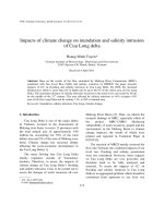
(Parmesan, 2006). A recent review has conceptualized the ways in which species can
react to changes in climate by considering the movement of their niche along three axes:
time (phenological change), space (distributional change) and self (physiological
change) (Bellard et al., 2012, Figure 1.1). Theoretically, where populations or species
fail to adapt or evolve along one or more of these axes, they will become locally or
globally extinct. Whilst local extinctions resulting from climate change have been well
documented (Franco et al., 2006, Parmesan et al., 1999, Sinervo et al., 2010), evidence of
global extinctions caused by climate change is present but scarce (Pounds et al., 2006).
That said, it has been proposed that the process of extinction due to climate change may
be time-delayed (Thomas et al., 2006) much like extinctions due to habitat
6

fragmentation (Tilman et al., 1994). An important prerequisite to extinction, though, is
population decline (Caughley, 1994).


Figure 1.1. Conceptual diagram from Bellard et al. (2012). Shown are three directions of biological
responses to cope with climate change. Axes represent movements in space (e.g. widespread latitudinal
range shifts (Hickling et al., 2006)), time (e.g. advanced leafing and flowering dates (Menzel et al., 2006))
and self (e.g. physiological changes in tropical fishes (Johansen & Jones, 2011)).

1.2. Mechanisms by which climate change affects populations of species
Large populations of species of conservation concern are more desirable than small
populations; one reason for this is that the latter are at a higher risk of extinction due to
Allee effects (Brook et al., 2008). Even ignoring extinction risk, population size is an
7

important biodiversity metric with implications for ecosystem services (Mace, 2005).
Continued population declines occurring in many biological systems are considered to
be economically catastrophic (Balmford et al., 2002) and such changes may take a long
time to reverse, with the example of depleted stocks of marine fishes (Hutchings, 2000).
Furthermore, population declines in more familiar species can be of great concern to
the general public, as illustrated by Britain’s relationship with its breeding birds
(Greenwood, 2003, in Balmford et al. 2003). Climate change can heavily influence
biodiversity at the population level, and this has already happened through a variety of
mechanisms. Shifts along the “time” and “space” axes of Bellard et al. (2012) can be and
have been responsible for changes in species’ abundance. A failure to respond
adequately along these axes may also cause population declines, especially where
species interactions are altered in the process (Cahill et al., 2013).
The most common reports of biological responses to climate change concern
changes in species’ phenologies (Parmesan, 2006). Advances in timing of events such as
leafing, flowering and fruiting have been widespread, and these are correlated with
changes in temperature (Menzel et al., 2006). Phenological responses also occur in
animals, as exemplified by earlier egg laying dates of birds in the UK and North America
(Crick et al., 1997, Dunn & Winkler, 1999). A large scale study on the pied flycatcher
even claimed to establish a causal relationship between climate change and advances in
breeding dates (Both et al., 2004). These advances in egg-laying dates have led to
population declines; black grouse offspring are exposed to colder conditions with
earlier hatching, resulting in increased mortality and population declines (Ludwig et al.,
2006). In addition, climate change has led to mismatches in timing between birds

breeding and the peak abundance of food for nestlings (Visser & Both, 2005). Some
populations of the pied flycatcher have failed to match the advance in timing of the peak
abundance of their prey, and this has been linked to population declines of up to 90%
(Both et al., 2006). This may be common amongst migratory birds, as European species
which have failed to adjust their migration date are generally the same species that are
experiencing population declines (Moller et al., 2008). Clearly phenological responses to
climate change can strongly impact upon population size.
Climate change responses at the species level materialize not only through
changes in timing, but through movements in geographical space. Species’ boundaries
8

have largely shifted to higher latitudes and altitudes during recent global warming
(Thomas, 2010), demonstrating the importance of the relationship between climate and
the broad scale distribution of species (Jiménez-Valverde et al., 2011). Whilst many
studies report species’ range expansions to higher latitudes (Hickling et al., 2006, Hitch
& Leberg, 2007, Thomas & Lennon, 1999), range retractions at the low latitude
boundary are detected less frequently (Thomas et al., 2006). This is also the case for
altitudinal shifts; cold upper boundaries shifted upwards far more frequently than did
warm lower boundaries in tropical studies (Thomas, 2010). Range shifts have been
ascribed to local extinction gradients, whereby the ratio of extinctions to colonizations
is greater at the warm range margin than at the cool range margin (Franco et al., 2006,
Parmesan et al., 1999). Under these conditions, if there is a lack of suitable habitat at the
expanding range margin, species’ ranges may be prevented from expanding (Hill et al.,
1999) and as such might contract overall. Given the established relationship between
species’ abundance and range size (Brown, 1984), it follows that expansions and
contractions will be associated with population increases and declines. Although
paleoecological studies reveal that range expansions and contractions have occurred in
response to climate for tens of thousands of years, the dispersal ability of species is now
heavily limited across habitats fragmented by human activity (Dawson et al., 2011). For
this reason, movements of species’ ranges could result in expansions, but also

retractions and population declines.
A recent meta-analysis found that as well as abiotic changes, changing species
interactions are a prominent factor affecting species populations under climate change
(Cahill et al., 2013). Direct climate induced impacts on prey or pathogens can be a
mechanism for population change, and may be considered distinct from mismatches in
species interactions caused by phenological change (Cahill et al., 2013). For example,
declines in the golden plover in the UK have been attributed to reduced abundance of
their cranefly prey resulting from high summer temperatures (Pearce-Higgins et al.,
2010). Conversely, declines in frogs of the genus Atelopus were caused by the spread of
a fungal pathogen which was facilitated by climate change (Rohr & Raffel, 2010). Where
climate change improves species’ chances of colonization and establishment in foreign
environments, new invasive species could emerge (Hellmann et al., 2008) with possible
consequences for native populations (Roy et al., 2012). There are also concerns that
9

existing alien species may increase their invasive potential if climate change enhances
their competitive ability (Peterson et al., 2008, Thuiller, 2007). Examples where climate
indirectly affects populations through species interactions appear as frequently as those
with direct abiotic causes (Cahill et al., 2013).

1.3. Biodiversity Indicators for Conservation and Policy
Many governments have pledged through the Convention on Biological Diversity to
reduce the rate of biodiversity loss by 2010, and this has signified their
acknowledgement of the value of biodiversity for human welfare (Balmford et al.,
2005). A variety of biodiversity indicators have been developed to assess progress
towards this broad target; these measure pressures on biodiversity (e.g. climate
change), the state of biodiversity metrics (e.g. population size), and the degree of
political response to biodiversity loss (Mace & Baillie, 2007). A study by Butchart et al.
(2010) collated a number of indicators to produce a timely evaluation of the
achievement of the 2010 target, and found that the rate of biodiversity loss had not

significantly decreased. In fact, indicators of biodiversity pressures had actually
increased overall (Butchart et al., 2010). This study demonstrated how broad
biodiversity indicators can be used to assess conservation efforts, whilst others
demonstrate a capacity for indicators to inform policy decisions at a more local scale
(Nicholson et al., 2012).
Despite the clear utility of indicators, there are still many aspects of biodiversity
conservation which have not been covered by efforts to date (Walpole et al., 2009).
Spatial, temporal and taxonomic biases impede the robustness of indicators, and this
could be improved in order to assess more specific targets in future (Butchart et al.,
2010, Jones et al., 2011, Mace et al., 2010). In addition, many indicators have arisen
primarily because of data availability, and not their rigorous methods or biodiversity
relevance (Mace & Baillie, 2007). Biodiversity indicators are not greatly informative
when presented alone, and should be complimented by a detailed understanding of
underlying ecological factors (Gregory et al., 2005). For an indicator to be any use at all,
though, it must be designed such that it is suitable for its function.
10

The gap between scientists and policymakers may have hampered conservation
efforts in the past (Mooney & Mace, 2009), and in order to effectively bridge this gap an
indicator must be clear and methodologically sound (Mace & Baillie, 2007). In the
interests of clarity an indicator should state which attribute of biodiversity it
represents, and whether it measures a biodiversity pressure, state, or response (Mace &
Baillie, 2007). It is also important to determine the extent to which the indicator is
intended to represent biodiversity as a whole (Gregory et al., 2005). Once the purpose
of the indicator is clearly defined, appropriate data and methods must be implemented
in its design. For example, gaps or biases in the data should be accounted for, and the
relationship between the indicator and biodiversity in general should be substantiated
(Gregory et al., 2005). Money, time and expertise are always finite, so a more practical
indicator is always desirable (Gregory et al., 2005).
Examples of headline indicators of the state of biodiversity that were analyzed by

Butchart et al. (2010) include a Wild Bird Index, which comprises aggregated
population trends for habitat specialist birds across Europe and North America. The
Climatic Impact Indicator for European birds developed by Gregory et al. (2009) is an
example of an indicator of a pressure on biodiversity, because population change is
linked to a single driver. An example of an indicator of political response to biodiversity
declines is the coverage of protected areas over time (Butchart et al., 2010), which
represents the extent of action taken by authorities to prevent further declines.
Examples such as these, whilst they are imperfect, are informative at the broadest scale.
Indicators represent a conduit through which the most politically relevant information
on biodiversity can be presented to and understood by non-scientists.

1.3.1. Using Birds to Represent Biodiversity
A large proportion of the information available to assess biodiversity change
corresponds to the distributions and populations of avian species. Owing to the
continued popularity of birds amongst the general public, these data are also being
collected more widely and thoroughly over time (Greenwood, 2007, Gregory et al.,
2005). Regional surveys of bird populations are unmatched in scale by surveys on other
species groups, and the best examples of these include the North American Breeding
11

Bird Survey (BBS) (Pereira & David Cooper, 2006). Around 2,500 of over 5,100
roadside survey routes across North America are surveyed each year, providing data for
over 420 bird species (Sauer & Link, 2011). Information from the BBS has been useful
to understand patterns in bird populations across both space and time, as well as to
monitor invasive species (NABCI, 2011, Robbins et al., 1986). Just one example of the
usefulness of this huge dataset is the analysis of the causes of declines in the majority of
North American grassland birds (Peterjohn & Sauer, 1999). Other examples have
involved tracking direct and indirect effects of pathogens on bird populations (LaDeau
et al., 2007, Nocera & Koslowsky, 2011). To account for problems such as observer bias
that exist in data from the BBS (Link & Sauer, 1998, Sauer et al., 1994), more precise

population trend estimates are now being derived using hierarchical models rather than
route-regression (Link & Sauer, 2002, Sauer & Link, 2011). Data from large scale bird
surveys have had an impact upon policy in the UK (Greenwood, 2003), indicating the
importance of such schemes in the context of biodiversity conservation. In addition,
population trends have been used to measure the benefits of conservation policy in
Europe (Donald et al., 2007) showing that long term BBS data is useful not only to
inform conservation policy, but to evaluate it.
Birds are a highly appropriate study taxon when investigating species responses
to climate change; this group has shown a marked reaction to changing climates across
many species and geographical regions (e.g. Crick, 2004, Hitch & Leberg, 2007, Thomas
& Lennon, 1999). There is a relationship between the broad scale distribution of birds
and climatic variables (Araújo et al., 2009, Jiménez-Valverde et al., 2011) although the
strength of this relationship has been contested (Beale et al., 2008, Beale et al., 2009, but
see Peterson et al., 2009). This relationship, as well as the dispersive ability of most
birds, may go some way towards explaining the ubiquity of avian distributional
responses to climate change. Phenological responses by birds are also widespread
(Crick, 2004) as exemplified by advanced egg laying dates in many species (Crick et al.,
1997, Dunn & Winkler, 1999). Distributional and phenological changes result in
altered species interactions (Cahill et al., 2013), which suggests that climate change
responses in birds will affect other taxa and vice versa. It is important to document and
understand these signal responses to gauge not only how birds react to climate change,
but how other components of biodiversity might do so. Studies projecting avian
12

responses under future climate change are prevalent (Matthews et al., 2004) and often
predict that ranges of the majority of species will decrease (Barbet-Massin et al., 2012,
Jetz et al., 2007). These predictions may also be alarming for other species groups,
although this depends on the extent to which birds can represent biodiversity as a
whole.
Recent studies assessing the use of bird species richness to predict the richness

of other groups suggest that birds do not always make suitable biodiversity indicators
(Eglington et al., 2012). However, as well as testing spatial relationships between
diversity of birds and of other taxa, it is important to consider whether temporal change
in assemblages of birds reflects changes in other groups (Favreau et al., 2006). Birds
tend to be near the top of the food chain, and as a result it is thought that they are highly
responsive to changes in their biotic environment (Gregory et al., 2005). This might
explain the evidence that links population trends in birds with trends in other taxa;
many studies have shown declines of farmland birds in parallel with declines in other
groups, especially invertebrates, resulting from agricultural intensification (Benton et
al., 2002, in Gregory et al., 2005, Robinson & Sutherland, 2002). In light of such
evidence, Gregory et al. (2005) argue that their farmland bird population index might
hold some value as a biodiversity indicator. However, it is not uncommon for some
species groups to respond negatively to a driver of biodiversity change whilst others
respond positively, so there is always a need for caution when using one species group
to represent many others. Whilst birds may not always be able to represent biodiversity
as a whole, they are important in their own right owing to their role in ecosystem
services such as pest control and seed dispersal (Whelan et al., 2008). Indicators of
population trends in bird species are important for conservation policy even if they are
not representative of trends in other taxa.

1.4. Species distribution modeling in the context of climate change
The applications of Species Distribution Models (SDMs) are extremely diverse, ranging
from spatial conservation planning to discovery of new populations of species (Araújo &
Peterson, 2012). One of the most popular uses of SDMs is to predict future effects of
climate change on biodiversity (e.g. Thomas et al. 2004). Thomas et al. (2004) used
13

SDMs to predict the change in range size of a variety of taxa under climate change with
two extreme dispersal scenarios and predicted that 15-37% of taxa within the study
area would be committed to extinction by 2050. Whilst such studies have been

criticized in light of the variability between different modeling processes (Thuiller et al.,
2004) and possible misrepresentation of results through sensationalist media (Ladle et
al., 2004), they highlight the utility of SDMs to speculate future impacts of climate
change on biodiversity. SDMs rarely take into consideration biotic interactions, species
dispersal or evolutionary change (Pearson & Dawson, 2003). In light of this, whilst
models may be useful for asking ‘what if’ questions, it is important not to place too
much faith in their projections as reliable predictions for the future (Araújo et al., 2005).
When analyzing species distributions with regard to climate change, SDMs often
focus on establishing the ‘bioclimate envelope’ of a species (Pearson & Dawson, 2003).
The bioclimate envelope may be determined in two main ways: by correlating a species’
current distribution with climate variables (the correlative approach), or by
understanding a species’ physiological responses to changes in climate (the mechanistic
approach) (Hijmans & Graham, 2006). A variety of model classes are commonly used to
calculate the bioclimate envelope, amongst them Generalized Linear Models (GLM),
Generalized Additive Models (GAM), Classification Tree Analyses (CTA) and Artificial
Neural Networks (ANN) (Thuiller, 2004). In fact, recently adopted modeling methods
such as machine learning have been shown to outperform older ones (Elith et al., 2006).
Once the climate envelope of a species has been determined, resultant models may be
applied to future climate scenarios to project the potential future distribution of that
species (e.g. Huntley et al., 1995). However, there is a high level of variability between
the broad range of common modeling techniques (Pearson et al., 2006, Thuiller, 2003,
Thuiller, 2004) and climate change scenarios (Thomas et al., 2004).
To account for such uncertainty, a process termed ‘ensemble forecasting’ has been
proposed; this involves making projections using a range of different models and
scenarios to produce more robust forecasts (Araújo & New, 2007). A suggested
platform for this process is BIOMOD (Thuiller et al., 2009), a package implemented in
the statistical analysis program R (R Development Core Team, 2012). BIOMOD offers a
convenient and accessible means to project species distributions, as it has options to
include a variety of model classes, validation methods and climate scenarios (Thuiller et
14

al., 2009). However, even when using ensemble forecasting, projections are dependent
on both the species analyzed and the classes of model used (Thuiller, 2003, Thuiller,
2004). This necessitates validation of SDMs before reaching any sound conclusions from
them.
Validation of SDMs may be carried out using three main methods: resubstitution,
data partitioning and using independent data. Resubstitution is the process whereby
models are validated using the same data which was used to calibrate them (Araújo et
al., 2005). Resubstitution has the fault that if a model overfits to the calibration data,
validating it against the same data may misrepresent the model’s accuracy when
predicting independent data (Araújo et al., 2005). Partitioning of the data to emulate an
independent data set (often splitting data 70:30, e.g. Thuiller, 2003, Thuiller, 2004)
assumes that random samples from the original data constitute independent samples
(Araújo et al., 2005). This is not true; both resubstitution and data partitioning fail to
account for spatial autocorrelation or temporal correlation in species distributions and
climate variables (Araújo et al., 2005). It has been shown that validating models using
non-independent data (i.e. resubstitution or data partitioning) produces over optimistic
estimates of model accuracy when compared to validation using independent data
(Araújo et al., 2005). Whilst rarely available, independent data is desirable when
validating SDMs. One way to obtain such data is from known distributions of the study
species in different regions (Peterson, 2003). Whilst models can still be useful without
truly independent data to validate them, this is contingent on their appropriate use and
acknowledgement of their assumptions and limitations (Araújo & Peterson, 2012).
SDMs often use presence-absence data for the distributions of species (Thuiller et
al., 2009), but models derived from these data can be used to make inferences with
regard to spatial patterns in species abundance (VanDerWal et al., 2009). There exists a
central tendency of species’ abundance in space, and it is thought that this is associated
with gradients in environmental suitability (Brown, 1984). SDMs allow an index of
environmental suitability to be derived by correlating present distributions of a species
with environmental variables, and this index can be used to predict species abundance

(Van Couwenberghe et al., 2012). Similar approaches have related modeled temporal
changes in climatic suitability for bird species to their recent population trends, offering
a form of validation for the use of SDMs in future projections (Green et al., 2008). In this
15

way, SDMs can be used not only to predict changes in biodiversity due to climate
change, but to retrodict them. Gregory et al. (2009) took this a step further and used the
relationship between trends in populations and climate suitability to produce a simple
climatic impact indicator for European bird populations from 1980-2005. However,
another study demonstrates that climate suitability is less able to predict population
stability, which is an important factor for long term population persistence (Oliver et al.,
2012). SDMs can be used to offer an indication of some population-level impacts of
recent climate change, but not all (Gregory et al., 2009).

1.5. Aims
In this project I will make use of two freely available and independent datasets relevant
to North American birds. Species distributions will be obtained from the BirdLife
International database (BirdLife International, 2013) and population trends will be
obtained from the North American Breeding Bird Survey (BBS) (Sauer et al., 2012).
Using the distribution dataset, I will produce species distribution models (SDMs)
relating the distributions of 384 avian species to bioclimate across North America.
These SDMs will then be used to derive two metrics of the relationship between a given
species and climate change: CST, which represents the slope of climatic suitability for a
species between 1968 and 2011, and CLIM, which represents whether a species’ range
is likely to increase or decrease by the end of the century under projected climate
change. Using these metrics, I will separate species into two groups – those expected to
benefit from climate change, and those expected to lose.
Using the population trends dataset, I will summarize overall population change for
each species between 1968 and 2011. Species level population trends will then be
merged based on the two groups produced using SDMs. If climate change has affected

avian populations since 1968, then species expected to benefit from climate change
might increase in abundance, whilst others decline. It is on this basis that climatic
impact indicators (CIIs) will be produced; these will compare population trends for the
two groups of species, such that an increase in a CII over time will mean that “climate
winners” have shown greater overall population increases than “climate losers” (Figure
16

1.2). The data used to produce SDMs and those used to produce population trends are
independent, and so this result would be consistent with a strong impact of climate
change on avian populations over the past half-century (Gregory et al., 2009). Two CIIs
will be produced for avian populations across mainland USA – one using CST to group
species and one using CLIM.
Following this, state-level CIIs will be produced in order to deconstruct the USA CII
and better understand climatic impacts on populations at more local scales. State-level
CIIs will then be merged, however, producing a novel “composite” USA CII. This will
offer a collective interpretation of climatic impacts on populations of avian species
across the USA whilst retaining the resolution of the state-level approach.
During the production of CIIs, I will explore how the model class used to relate a
species’ distribution to bioclimate affects the outcome of a CII. I will also determine the
outcome of using two different methods to classify species into those expected to be
positively or negatively affected by climate change. The spatial and temporal scale of the
study (first across the entire mainland USA, then at the state level, annually between
1968 and 2011) is often dictated by the availability of data on distributions and
population trends.
The indicators produced will fill an important geographical gap amongst indicators
on the pressure of recent climate change on biodiversity. This study will use similar
methods to Gregory et al. (2009) on a separate region covering a comparable range of
latitudes. This will bridge a significant geographical gap in current understanding of
population level climate change impacts, and establish whether the trends observed
across Europe are also occurring elsewhere. Using a novel method, I will also assemble

CIIs at the state level and combine them to produce a composite USA CII. In doing so, I
will optimize the production of simple CIIs that will ultimately be useful to monitor our
progress towards broad biodiversity targets (Mace & Baillie, 2007). This will help to
narrow the gap between scientists and policy makers in future (Mooney & Mace, 2009).



17


Figure 1.2. Flow diagram outlining the core stages of the production of a climatic impact indicator (CII).
18

2. Modeling Distributions of North American Bird Species Using
Bioclimatic Variables
2.1. Introduction
Global average temperatures have been rising rapidly over the past 50 years (IPCC,
2007) and as a consequence species distributions have shifted uphill and towards the
poles (Hickling et al., 2006, Thomas, 2010). This response has been widespread across
many taxa, demonstrating the significance of the broad scale association between
climate and species’ distributions (Jiménez-Valverde et al., 2011). Species distribution
models (SDMs) can make use of this relationship by correlating a species’ occurrence
with the climate found across its range (Pearson & Dawson, 2003). They may then be
used to predict that species’ distribution based on climate variables in a different time
or place. For this reason SDMs have a variety of applications, ranging from predicting
future effects of climate change on biodiversity (e.g. Thomas et al., 2004) to retrodicting
changes in population size based on climate suitability (Green et al., 2008). Gregory et
al. (2009) used SDMs to determine which European bird species were expected to be
positively or negatively affected by recent climate change. This allowed a comparison of
the population trends for these two groups, indicating how strongly recent climate

change has affected populations of European bird species.
In order to make inferences from SDM predictions, it is important that they are
adequately validated (Araújo et al., 2005). Wherever possible SDMs should be evaluated
using data that are independent of those used to calibrate them, but such data are rarely
available. As a compromise, individual SDMs can be validated in the absence of
independent data using the following methods:
Resubstitution: SDMs are validated using the same data that were used to
calibrate them. Predicted distributions based on the full calibration dataset are
compared with observed distributions. However, if a model overfits to the
calibration data, testing the model on the same data will misrepresent the
model’s accuracy (Araújo et al., 2005).
Data partitioning: The data are partitioned randomly to emulate an independent
dataset (often splitting data 70:30, e.g. Thuiller, 2003, Thuiller, 2004). A model
19

built with the calibration data (70%) is used to predict the remaining test data
(30%) in order to assess its performance. Whilst this approach is preferred to
resubstitution, it assumes that random samples from the original data constitute
independent samples (Araújo et al., 2005).
Both data partitioning and resubstitution fail to account for spatial autocorrelation or
temporal correlation in species distributions and climate variables (Araújo et al., 2005).
Although these methods are imperfect, they offer an indication of how an individual
model performs in the absence of independent data. Other methods exist to evaluate
individual model performance, for example spatial segregation of data through k-fold
partitioning (Bagchi et al., 2013). Alternatively, it is possible to use SDMs to predict
changes in abundance over time (Green et al., 2008), and this approach will be
considered in later chapters.
SDMs are useful not only to predict individual species’ distributions according to
climate, but to predict community properties such as species richness (Ferrier &
Guisan, 2006) and composition (Benito et al., 2013). This can be done by aggregating

SDM predictions for different species in the same region, creating what has been termed
stacked-species distribution models (S-SDMs, Guisan & Rahbek, 2011). Performance of
S-SDMs must be evaluated based on their ability to predict community properties in the
present; Benito et al. (2013) have suggested directly comparing observed and predicted
species richness in a given location, and using similarity indices such as the Sorensen’s
index to compare observed and predicted species composition (see Koleff et al., 2003).
By building and evaluating S-SDMs as well as SDMs, it is possible to determine not only
how well individual models perform, but how well a large number of such models
perform at the community level.
In this project, SDMs will be used to separate North American birds into groups of
species expected to be positively or negatively affected by climate change. By comparing
the multispecies population trends of these two groups, it will be possible to produce a
climatic impact indicator (CII) much like the European indicator produced by Gregory et
al. (2009). To this end, in this chapter I develop three classes of SDMs for 384 North
American bird species (listed in Appendix 1). Prior to making predictions from these
SDMs, it must be confirmed that they can adequately predict existing distributions. I test