Analysis and computation for coupling bose einstein condensates in optical resonators
Bạn đang xem bản rút gọn của tài liệu. Xem và tải ngay bản đầy đủ của tài liệu tại đây (10.15 MB, 80 trang )
Analysis and Computation for Coupling
Bose-Einstein Condensates in Optical Resonators
Xu Wei Biao
NATIONAL UNIVERSITY OF SINGAPORE
2010
Analysis and Computation for Coupling
Bose-Einstein Condensates in Optical Resonators
Xu Wei Biao
(B.Sc. Sun Yat-Sen University of China)
A THESIS SUBMITTED FOR THE DEGREE OF
MASTER OF SCIENCE
DEPARTMENT OF MATHEMATICS
NATIONAL UNIVERSITY OF SINGAPORE
2010
Acknowledgements
First of all, I would like to sincerely express my thanks to my supervisor, Prof Bao Weizhu
for his thoughtful kindness and priceless guidance. He gave me great encouragement and
help when I was in a maze and patiently led me to the right way in both research and
life.
Furthermore, many thanks go to my senior, Dr Wang Hanquan for nurturing my
mathematical maturity. He shared his valuable experience in research work and offered
me great help on my thesis.
I would also like to thank my family and friends, for their unconditional love and
support. Special thanks go to Zhou Fan, Sit Wing Yee, Goh Siong Thye, Dong Xuan
Chun, Wong Weipin, Tang Qinglin and Zhang Yong. It is my honor to have these friends.
Last not the least, I am grateful for the financial support from the National University of Singapore and Ministry of Education of Singapore. Without the scholarship
provided for me, I would not be able to pursue my dream in study.
Xu Wei Biao
Aug 2010
1
Contents
List of Tables
5
List of Figures
6
1 Introduction
9
1.1
Development of BEC . . . . . . . . . . . . . . . . . . . . . . . . . . . . . . 10
1.2
Numerical methods on single BEC . . . . . . . . . . . . . . . . . . . . . . 11
1.3
Contemporary studies in BEC . . . . . . . . . . . . . . . . . . . . . . . . . 12
1.4
The problem . . . . . . . . . . . . . . . . . . . . . . . . . . . . . . . . . . 13
1.5
Overview of this work . . . . . . . . . . . . . . . . . . . . . . . . . . . . . 14
2 Coupled BEC in optical resonators
16
2.1
Dimensionless formulation . . . . . . . . . . . . . . . . . . . . . . . . . . . 16
2.2
Reduction to lower dimensions . . . . . . . . . . . . . . . . . . . . . . . . 17
2.2.1
Reduction to 2D . . . . . . . . . . . . . . . . . . . . . . . . . . . . 17
2.2.2
Reduction to 1D . . . . . . . . . . . . . . . . . . . . . . . . . . . . 18
2.3
The general model . . . . . . . . . . . . . . . . . . . . . . . . . . . . . . . 19
2.4
Some conservation properties . . . . . . . . . . . . . . . . . . . . . . . . . 19
2.4.1
Mass conservation . . . . . . . . . . . . . . . . . . . . . . . . . . . 19
2.4.2
Energy conservation . . . . . . . . . . . . . . . . . . . . . . . . . . 21
3 Ground state of coupling BEC in optical resonators
23
3.1
Stationary solutions . . . . . . . . . . . . . . . . . . . . . . . . . . . . . . 23
3.2
Ground state . . . . . . . . . . . . . . . . . . . . . . . . . . . . . . . . . . 24
3.3
Numerical method . . . . . . . . . . . . . . . . . . . . . . . . . . . . . . . 26
2
CONTENTS
3.4
3.3.1
Continuous normalized gradient flow . . . . . . . . . . . . . . . . . 26
3.3.2
Gradient flow with discrete normalization . . . . . . . . . . . . . . 27
3.3.3
A backward Euler Sine pseudospectral method . . . . . . . . . . . 29
Numerical results . . . . . . . . . . . . . . . . . . . . . . . . . . . . . . . . 30
3.4.1
Ground state solutions in 1D . . . . . . . . . . . . . . . . . . . . . 31
3.4.2
Ground state solutions in 2D . . . . . . . . . . . . . . . . . . . . . 35
4 Dynamics of coupling BEC in optical resonators
4.1
41
Dynamical laws . . . . . . . . . . . . . . . . . . . . . . . . . . . . . . . . . 41
4.1.1
Dynamical laws for the condensate width . . . . . . . . . . . . . . 42
4.2
Time-splitting Sine pseudospectral methods . . . . . . . . . . . . . . . . . 46
4.3
Accuracy tests
4.4
. . . . . . . . . . . . . . . . . . . . . . . . . . . . . . . . . 54
4.3.1
Accuracy tests in 1D . . . . . . . . . . . . . . . . . . . . . . . . . . 54
4.3.2
Accuracy tests in 2D . . . . . . . . . . . . . . . . . . . . . . . . . . 56
4.3.3
Conservation of dynamics properties . . . . . . . . . . . . . . . . . 57
Numerical results . . . . . . . . . . . . . . . . . . . . . . . . . . . . . . . . 57
4.4.1
1D dynamical cases . . . . . . . . . . . . . . . . . . . . . . . . . . . 58
4.4.2
2D Dynamical cases . . . . . . . . . . . . . . . . . . . . . . . . . . 61
5 Conclusion
69
3
CONTENTS
Summary
Since 1995, Bose-Einstein condensates (BEC) of alkali atoms have been produced and
studied extensively in experiments. One central goal of experiments has been formation
of Bose-Einstein condensates with a number of atoms as large as possible. Based on mean
field theory, Jaksch et al. recently proposed a mathematical model—Gross-Pitaevskii
equations coupled with an integral and ordinary differential equation in order to study
the possibility of how to unite two BEC in optical resonators. However, the authors
investigated this possibility through two-mode analysis of the mathematical model. In
this thesis, we propose efficient numerical methods—Sine pseudospectral methods to
solve the mathematical model and perform direct numerical simulations on studying
such possibility.
We first investigate the ground state solutions of two coupling BEC, which describe
the equilibrium state of the coupling BEC in optical resonators at extremely low temperature. We compute the ground state solutions by proposing a normalized gradient flow
discretized with backward Euler Sine pseudospectral approach. We use our numerical
one-dimensional and two-dimensional solutions to study which factors may be useful for
uniting BEC in optical resonators at equilibrium.
We next study the dynamics of two coupling BEC in optical resonators by designing new efficient numerical methods—time-splitting Sine pseudospectral methods for the
Gross-Pitaevskii equations coupled with an integral and ordinary differential equation.
Though there is an extra ordinary differential equation with integral term in the mathematical model for the dynamics of coupling BEC in optical resonators, which may bring
us some numerical difficulties, we successfully adapt the usual time-splitting methods
to deal with them. The proposed numerical methods keep the dynamical properties of
the mathematical model very well in the discretized level and have spectral accuracy in
space. The numerical results obtained by these efficient numerical methods are used to
analyze the possible way of dynamically uniting BEC in optical resonators.
4
List of Tables
4.1
Temporal error analysis for TSSP1 in 1D: errors at t=5.0 with ∆x =
1
32
. 55
4.2
Temporal error analysis for TSSP2 in 1D: errors at t=5.0 with ∆x =
1
32
. 55
4.3
Spatial error analysis for TSSP1 in 1D: errors at t=5.0 with ∆t = 0.0001.
55
4.4
Spatial error analysis for TSSP2 in 1D: errors at t=5.0 with ∆t = 0.0001.
56
4.5
Temporal error analysis for TSSP1 in 2D: errors at t=5.0 with ( x,
1 1
32 , 32
4.6
. . . . . . . . . . . . . . . . . . . . . . . . . . . . . . . . . . . . . . 56
Temporal error analysis for TSSP2 in 2D: errors at t=5.0 with ( x,
1 1
32 , 32
y) =
y) =
. . . . . . . . . . . . . . . . . . . . . . . . . . . . . . . . . . . . . . 56
4.7
Spatial error analysis for TSSP1 in 2D: errors at t=5.0 with ∆t = 0.0001.
57
4.8
Spatial error analysis for TSSP2 in 2D: errors at t=5.0 with ∆t = 0.0001.
57
5
List of Figures
1.1
Velocity-distribution data of rubidium-87. From temperature T1 to T3,
the temperature becomes lower and lower. T1 is the temperature before
the appearance of a BEC; at T2, the condensate appears; and at T3,
nearly pure condensate is formed. (taken from Wikipedia). . . . . . . . . .
1.2
(a) Experiment setup, (b) Level structure. (taken from [27]).
3.1
Gradient flows prepared with different initial data converge into the same
9
. . . . . . . 13
steady-state solution which has the same energy. . . . . . . . . . . . . . . 31
3.2
Density plots of ground states trapped in a harmonic trap with different
coupling strength g in Example 3.2.
3.3
Density plots of ground states trapped in a double-well trap with different
coupling strength g in Example 3.2.
3.4
. . . . . . . . . . . . . . . . . . . . 32
. . . . . . . . . . . . . . . . . . . . 33
Density plots of ground states of coupling BEC trapped in an optical
lattice trap with different coupling strength g in Example 3.2.
3.5
Masses of two condensates in the harmonic trap, i.e., N (ψ), N (φ) for
different coupling strength g in Example 3.2.
3.6
. . . . . 34
. . . . . . . . . . . . . . . 35
Masses of two condensates and photons (i.e., N (ψ) N (φ) N (C)), energy
E and chemical potential µ of the ground states for different interaction
parameter β. . . . . . . . . . . . . . . . . . . . . . . . . . . . . . . . . . . 36
3.7
Masses of two condensates and photons (i.e., N (ψ) N (φ) N (C)), energy
E and chemical potential µ of the ground states for different detuning
strength δ1 . . . . . . . . . . . . . . . . . . . . . . . . . . . . . . . . . . . . 37
6
LIST OF FIGURES
3.8
Gradient flows prepared with different initial data converge into the same
steady-state solution which has the same energy in Example 3.4
3.9
. . . . 38
Density plots of ground states of coupling BEC in the harmonic traps (a)
with no shifts of centers in x-direction, and (b) with shifts a1 = −2 and
a2 = 2.
. . . . . . . . . . . . . . . . . . . . . . . . . . . . . . . . . . . . . 39
3.10 Density plots of ground states of coupling BEC in the double well trap
(a) with no shift (a3 = 0), and (b) with the shift a3 = 2.
. . . . . . . . . 39
3.11 Density plots of ground states of coupling BEC in different optical lattice
trap potentials V1 (x, y) = V2 (x, y) = 12 (x2 + y 2 ) + p(sin2 (qx) + sin2 (qy))
:(a) p=20,q=1; (b)p=20,q=2; (c)p=60,q=1; (d)p=60,q=2;
4.1
. . . . . . . . 40
(a)Conservation of energy and the total mass of two condensates in 1D.
(b)Conservation of energy and the total mass of two condensates in 2D. . 58
4.2
(a): Time evolution of the total condensate width in 1D. (b) time evolution
of the total condensate width in 2D. . . . . . . . . . . . . . . . . . . . . . 58
4.3
(a) time evolution of photons mass N(C) for different κ; (b) time evolution
of mass of ψ for different κ . . . . . . . . . . . . . . . . . . . . . . . . . . . 59
4.4
Time evolution of mass of two condensates when different g are applied
at time t = 0.
N (ψ)
N (φ)
. . . . . . . . . . . . . . . . . . . . . . . . . . . . . . . . . 60
4.5
Ratio
against g after t = 100. . . . . . . . . . . . . . . . . . . . . . . 61
4.6
Time evolution of mass of two condensates when different δ1 are applied
at time t = 0.
N (ψ)
N (φ)
. . . . . . . . . . . . . . . . . . . . . . . . . . . . . . . . . 62
4.7
Ratio
4.8
Time evolution of mass of two condensates when different Ω are applied
against δ1 after t = 200. . . . . . . . . . . . . . . . . . . . . . . 63
at time t = 0.
4.9
Ratio
N (ψ)
N (φ)
. . . . . . . . . . . . . . . . . . . . . . . . . . . . . . . . . 64
against Ω after t = 100.
. . . . . . . . . . . . . . . . . . . . . 64
4.10 Density plots of the ground states solutions, which are used as initial data
for studying the dynamics in 2D. . . . . . . . . . . . . . . . . . . . . . . . 65
4.11 (a) Time evolution of mass of two condensates: (a) g = 0.5; (b) g = 5. . . 65
4.12 Density plots for the wave-functions at t = 30: (a) g = 0.5; (b)g = 5. . . . 66
4.13 Time evolution of mass of two condensates: (a) δ1 = 0.5; (b) δ1 = 2. . . . 66
7
LIST OF FIGURES
4.14 Density plots for the wave-functions at t = 50: (a) δ1 = 0.5; (b) δ1 = 2.
4.15 Time evolution of mass of two condensates: (a) Ω = 0.1; (b) Ω = 2.
. 67
. . . 67
4.16 Density plots for the wave-functions at t = 200: (a) Ω = 0.1; (b) Ω = 2. . 68
8
Chapter 1
Introduction
The Bose-Einstein condensate (BEC) is a state of interacting bosons, which is cooled
to the temperature close to absolute zero (−273.15◦ C). Under such strict condition, a
large part of bosons will condense into the lowest energy state, which is the so called
quantum mechanical ground state (cf. Figure 1.1). In this chapter, we first introduce
brief history of the development of BEC, and then we review some theoretical studies
of single-component BEC. Finally we introduce recent development of BEC and our
problem to be investigated in the thesis.
Figure 1.1: Velocity-distribution data of rubidium-87. From temperature T1 to T3, the
temperature becomes lower and lower. T1 is the temperature before the appearance of
a BEC; at T2, the condensate appears; and at T3, nearly pure condensate is formed.
(taken from Wikipedia).
9
1.1. DEVELOPMENT OF BEC
1.1
Development of BEC
Based on a statistical description of photons done by an Indian physicist Satyendra Nath
Bose (1924) [3], a phenomenon was predicted by Einstein (1925) [20] that a BEC could
occur in a gas of noninteracting atoms below some critical temperature in the form of
phase transition.
In 1938, Pyotr Kapitsa, John Allen and Don Misener discovered superfluid from
helium-4 below temperature 2.17K, whose superfluidity was due to partial BEC of the
liquid. Later F. London showed that the superfluidity could be a manifestation of the
BEC. However, because of the limitation of technique, only a small fraction of condensate
was found in the experiments on superfluid till 1955. While in the 1970s, the BEC was
almost achieved when studies on dilute atomic gases were set up, but it was still not
pure [47].
With the development of laser and magnetic evaporative cooling techniques, the
first pure BEC, in vapors of rubidium-87 (cf. Figure 1.1) and sodium-23, was observed
separately by Eric Cornell, Carl Wieman at JILA and by Ketterle at MIT on 1995. Later,
it was achieved on many other atoms such as helium-4, rubidium-85 and spin-polarized
hydrogen.
New developments in dilute atomic gas unveiled remarkable properties of the BEC
[67]. The most remarkable one is the so-called wave-like behavior of matter, which is
shown on a macroscopic scale due to condensation of a large number of identical atoms
into the same quantum state. If the interactions between particles are weak in a dilute
atomic gas, the wave-like condensate can be summed up and described by a single particle
to show an average effect. This gives rise to the macroscopic wave function ψ(x, t) whose
evolution is governed by a self-consistent, mean field nonlinear Schrödinger equation
known as the Gross-Pitaevskii equation (GPE) [23, 46]
i
∂ψ(x, t)
∂t
=
δE(ψ)
δ ψ¯
2
= −
2m
∇2 ψ(x, t) + V (x)ψ(x, t) + U |ψ(x, t)|2 ψ(x, t),
where x = (x, y, z)T is the spatial coordinate vector;
10
(1.1)
is the Planck constant; ψ¯ is
1.2. NUMERICAL METHODS ON SINGLE BEC
the conjugate of ψ; m is the atomic mass; V (x ) is an external trapping potential;
U =
4π
2a
m
s
describes the interactions between atoms in the condensate; as is atomic
scattering length. The energy of the system E(ψ) can be defined as
2
E(ψ) =
R3
1.2
2m
|∇ψ(x, t)|2 + V (x)|ψ(x, t)|2 +
U
|ψ(x, t)|4 dx.
2
(1.2)
Numerical methods on single BEC
Numerical studies on single BEC models mostly concentrate on finding ground states and
simulating dynamical process via GPE (1.1). These studies provide powerful tools for
subsequent researches on BEC. In this section, we review the main numerical methods
for solving the GPE (1.1) in the study of single BEC.
To compute the ground state, there are two kinds of schemes: (i) finite difference
scheme, and (ii) pseudospectral scheme. In the former, Edwards and Burnetts [21]
introduced a Runge-Kutta method to solve GPE for 1D ground state and 3D ground state
with spherical symmetry; Bao and Du [5] proposed a backward Euler finite difference
method to discretize continuous normalized gradient flow with diminishing energy; and
Ruprecht et al. [50] presented a Crank-Nicolson finite difference method. For the latter
scheme, Bao et al. [7, 9] introduced a sine pseudospectral method to discretize continuous
normalized gradient flow for computing ground state. Each of these two schemes has
its advantages and disadvantages. The finite difference scheme is only of second order
spatial accuracy although it is implicit and unconditionally stable, while pseudospectral
scheme is of spectral accuracy in space, but it is conditionally stable [67].
To study the dynamics of the BEC, we can classify the methods into two groups:
(i) the finite difference methods which include Crank-Nicolson finite difference method
[50], alternating direction implicit method [57] and explicit finite difference method [17];
(ii) the pseudospectral methods which include the TSSP [6, 7] and Runge-Kutta pseudospectral method [2, 36]. These two kinds of methods are vastly applied in physical and
mathematical literatures. In numerical computation, we favor pseudospectral methods
rather than the finite difference methods since pseudospectral methods have high-order
accuracy.
11
1.3. CONTEMPORARY STUDIES IN BEC
1.3
Contemporary studies in BEC
With the development of technologies in experiments, various aspects of BEC have been
investigated. Quantized vortices in a BEC are recently obtained in experiments by
several groups, e.g. the JILA [35], ENS [34, 49] and MIT [48]; Another important
recent development in BEC was the study of spin-1 and spin-2 condensates. The spin-1
BEC was realized in experiments by using both sodium-23 and rubidium-87. BEC with
multiple species have also been achieved in experiments [25, 24, 30, 37, 52]. In addition,
the first experiment of two-component BEC was performed in JILA [37], and extensive
studies on multiple-component BEC have been carried out. The experimental progress
in BEC has greatly propelled the theoretical studies on BEC.
Subsequent numerical simulations and theoretical studies on BEC illustrated existent
experimental results in recent years. For a non-rotating BEC, Lundh et. al [33] investigated free expansion of vortex state, Bao and Du [5] computed central vortex states;
For a rotating BEC, several groups e.g. Bao et. al [6, 11], Jackson et. al [28, 29], and
Caradoc-Davis et. al [15, 16], simulated generation of vortices from the ground state
and studied dynamics of vortices, Svidzinsky and Fetter [55] investigated dynamics of
a vortex line which depends on its curvature, Modugno et. al [38] and Aftalion et. al
[1] presented bent vortices like S-shaped and U-shaped vortex, and compared with experimental results [49]; A spin-F BEC was described by the coupled GPEs [47, 46, 23],
and dynamical laws of the coupled GPEs for spin-1 BEC were proposed by Bao and
Zhang [12], while Wang [61] presented dynamics of spinor F=1 BEC. Moreover, Bao
[4] provided a mathematical justification by computing ground states and dynamics of
multi-component BEC, Lieb and Solovej [31] investigated the ground state energy of the
two-component charged Bose gas, Wang [62] presented numerical simulations on stationary states for rotating two-component Bose-Einstein condensates while Bao et al. [13]
computed the dynamics.
Although tremendous simulation results have been carried out, there are still lots of
challenging theoretical problems for multi-component BEC. One recent goal of physical
experiments is to form BEC with the numbers of atoms as large as possible. Therefore,
it is particularly interesting to realize the goal by forming a large single BEC via uniting
12
1.4. THE PROBLEM
two or more independent condensates.
1.4
The problem
Recently Jaksh et al. proposed that two initially independent BEC could be united to
one large BEC by putting them into a ring cavity and coupling them with an internal
Josphson junction [27, 64]. The experiment setup of the proposal are (cf. Figure 1.2(a)) :
Two initially independent condensates 1 and 2 trapped in a ring cavity are coupled with
two lasers Ω and Ω1 as well as the cavity mode. The Level structures of the experiments
are (cf. Figure 1.2(b)): Atoms are transferred by Raman laser Ω from level |1 > to
level |2 >. Another transition between particles in level |1 > and an auxiliary level
|3 > is drived by laser Ω1 . The cavity couples the levels |3 > and |2 > with the coupling
strength gc . In this experimental setup, the two condensates are trapped in many optical
resonators [64].
Figure 1.2: (a) Experiment setup, (b) Level structure. (taken from [27]).
According to the mean field theory, at extremely low temperature, the mathematical
model for describing the above-mentioned coupling BEC in optical resonators is the
13
1.5. OVERVIEW OF THIS WORK
following coupled equations [25, 27, 64]
i
∂ψ(x, t)
∂t
2
= −
2m
∇2 ψ(x, t) + V1 (x)ψ(x, t) + u11 |ψ(x, t)|2 + u12 |φ(x, t)|2 ψ(x, t)
+ (ˆ
g C(t) +
i
∂φ(x, t)
∂t
2
= −
2m
∂C(t)
∂t
(1.3)
∇2 φ(x, t) + V2 (x)φ(x, t) + u21 |φ(x, t)|2 + u22 |ψ(x, t)|2 φ(x, t)
¯ +
+ (ˆ
g C(t)
i
ˆ
Ω
)φ(x, t) + δˆ1 ψ(x, t),
2
ˆ
Ω
)ψ(x, t) + δˆ2 φ(x, t),
2
(1.4)
¯ t)ψ(x, t)dx + vˆC(t), x ∈ R3 , t > 0.
gˆφ(x,
=
(1.5)
R3
Here, ψ(x, t), φ(x, t) denote two wave functions of two coupling condensates, |C(t)|2
represents number of photons in the cavity at time t, ujk =
4
2 πa
m
jk
(j, k = 1, 2) are
the interactions, ajk is the s-wave scatting length for interspecies, δˆk , k = 1, 2, is the
effective detuning strength of condensates and vˆ is the effective detuning strength of
ˆ is frequency, and gˆ is the coupling strength of the ring cavity mode.
the ring cavity, Ω
Vk (x), k = 1, 2, are the external trapping potentials and they take the form
Vk (x) =
m 2 2
2
2
z 2 , k = 1, 2,
y 2 + ωz,k
ωx,k x + ωy,k
2
if they are harmonic. (1.5) is also called mode equation which describes the property of
optical cavity.
In [27], the authors investigate how to unite two independent condensates into a
single one through two-mode analysis of the coupled equations (1.3)-(1.5) and Montecarlo simulations. In this thesis, based on direct numerical solutions of the coupled
equations (1.3)-(1.5), we study ground state and dynamics of coupling BEC in optical
resonators, which may shed light on how two independent condensates could be united
to one BEC.
1.5
Overview of this work
The structure of this thesis is as follows.
In Chapter 2, we simplify the model into a dimensionless form by rescaling the
parameters and then we reduce the three dimensional model into lower dimensional
14
1.5. OVERVIEW OF THIS WORK
models. Last we define the energy for the whole system and prove the conservation
properties of mass and energy.
In Chapter 3, we first define the ground state for our model. We then compute the
ground state by constructing a normalized gradient flow discretized with backward Euler
Sine pseudospectral approach. Lastly we investigate the ground state of coupling BEC
in optical resonators for 1D and 2D cases.
In Chapter 4, we start off by investigating dynamical laws and then we solve the
mathematical model by using time-splitting Sine pseudospectral methods for the coupled
equations. Though there is an ODE with integral term in the mathematical model for
the dynamics of coupling BEC in optical resonators, which may bring some difficulties in
practical computation, we successfully adjust the usual time-splitting methods to solve
the model. Next, we test the convergence of our schemes and observe various dynamics
of coupling BEC in optical resonators through intensive numerical simulations.
In Chapter 5, we draw some conclusions of this work and inspire some ideas on future
directions.
15
Chapter 2
Coupled BEC in optical resonators
In this chapter, we first reformulate the coupled equations (1.3)-(1.5) into a dimensionless
formulation. Furthermore, for simplification of our study, we reduce the dimensionless
three-dimensional coupled equations into two-dimensional coupled equations and onedimensional coupled equations, respectively. Last, we investigate some conservation
properties of coupled equations in optical resonators.
2.1
Dimensionless formulation
To derive the dimensionless formulation for equations (1.3)-(1.5), we introduce a0 =
3
3
mωx,1 ,
˜=
x
x
a0 ,
˜ x, t˜) =
t˜ = ωx,1 t, ψ(˜
a02 ψ(x,t)
√
,
N
˜ x, t˜) =
φ(˜
a02 φ(x,t)
√
,
N
C˜ =
√C ,
N
where N
denotes the total particle number.
Plugging the above notations into equations (1.3)-(1.5), and then removing ∼ from the
notations, we obtain the following dimensionless form
i
∂ψ(x, t)
∂t
i
∂φ(x, t)
∂t
i
∂C(t)
∂t
1
= − ∇2 ψ(x, t) + V1 (x)ψ(x, t) + β11 |ψ(x, t)|2 + β12 |φ(x, t)|2 ψ(x, t)
2
Ω
+ gC(t) +
φ(x, t) + δ1 ψ(x, t),
(2.1)
2
1
= − ∇2 φ(x, t) + V2 (x)φ(x, t) + β21 |ψ(x, t)|2 + β22 |φ(x, t)|2 φ(x, t)
2
¯ + Ω ψ(x, t) + δ2 φ(x, t),
(2.2)
+ g C(t)
2
¯ t)ψ(x, t)dx + vC(t),
g φ(x,
=
R3
16
(2.3)
2.2. REDUCTION TO LOWER DIMENSIONS
where βk,l =
4πak,l N
,
a0
g=
√
gˆ N
ωx,1 ,
Vk (x) =
with γα,k =
2.2
ωα,k
ωx,1
v=
vˆ
ωx,1 ,
δk =
δˆk
ωx,1 ,
Ω=
ˆ
Ω
ωx,1
and
1 2 2
2
2
γ x + γy,k
y 2 + γz,k
z 2 , k = 1, 2,
2 x,k
( α = x, y, z).
Reduction to lower dimensions
In this section we reduce the dimensionless coupled equations (2.1)-(2.3) into twodimensional coupled equations and one-dimensional coupled equations.
2.2.1
Reduction to 2D
If the condensation is disk-shaped, i.e. ωx,1 ≈ ωy,1 , ωz,1
ωy,2 , ωz,2
ωx,1 , ωx,1 ≈ ωx,2 , ωx,1 ≈
ωx,1 , then the three dimensional GPEs could be reduced to two-dimensional
GPEs under an assumption that the time evolution could not cause excitation along the
z-axis. Compared with those along x-axis and y-axis, the excitation along z-axis has
much larger energy, so we might set
where ψh (z) = (
i
γz,1 1 −
4
π ) e
ψ(x, y, z, t) = ψ1 (x, y, t)ψh (z),
(2.4)
φ(x, y, z, t) = φ1 (x, y, t)φh (z),
(2.5)
γz,1 2
z
2
, φh (z) = (
γz,2 1 −
4
π ) e
γz,2 2
z
2
. We plug (2.4)-(2.5) into (2.1),
∂ψ1
1
1
ψh = − ∆ψ1 ψh − ψ1 (ψh )zz + V1 (x)ψ1 ψh + (β11 |ψ1 |2 |ψh |2
∂t
2
2
+β12 |φ1 |2 |φh |2 )ψ1 ψh + δ1 ψ1 ψh .
(2.6)
Multiplying (2.6) by ψh and integrating it with respect to z, we can obtain a new function
via some calculations
i
∂ψ1 (x, t)
∂t
1
= − ∇2 ψ1 (x, t) + V1 (x)ψ1 (x, t) + β˜11 |ψ1 (x, t)|2 + β˜12 |φ1 (x, t)|2 ψ1 (x, t)
2
Ω
+(gC(t) + )λ1 φ1 (x, t) + (δ1 + λ2 )ψ1 (x, t),
(2.7)
2
17
2.2. REDUCTION TO LOWER DIMENSIONS
γz,1
2π ,
where we denote β˜11 = β11
2
γz,1
− 21 (ψh (z)zz ψh (z)) +
R
2
1
(γz,1 γz,2 )
π(γz,1 +γz,2 ) ,
β˜12 = β12
(4γz,1 γz,2 ) 4
√
γz,1 +γz,2
λ1 =
, λ2 =
z 2 ψh (z)2 dz = 34 γz,1 .
Similarly, we can obtain two-dimensional coupled equations from (2.2)-(2.3) by setγz,2
2π ,
ting β˜22 = β22
∂φ1 (x, t)
∂t
i
i
∂C(t)
∂t
β˜21 = β21
(γz,1 γz,2 )
π(γz,1 +γz,2 ) ,
λ3 = 34 γz,2 ,
1
= − ∇2 φ1 (x, t) + V2 (x)φ1 (x, t) + β˜21 |ψ1 (x, t)|2 + β˜22 |φ1 (x, t)|2 φ1 (x, t)
2
¯ + Ω )λ1 ψ1 (x, t) + (δ2 + λ3 )φ1 (x, t),
+(g C(t)
(2.8)
2
=
R2
gλ1 φ¯1 (x, t)ψ1 (x, t)dx + vC(t).
(2.9)
Here, V1 (x) = V2 (x) = 12 (x2 + y 2 ).
2.2.2
Reduction to 1D
If ωx,1 ≈ ωx,2 , ωz,1
where ψh1 (y) = (
(
γz,2
π )
1
4
γ
− z,2
z2
2
e
ωx,1 , ωy,1
ωx,1 , ωy,2
ωx,1 , ωz,2
ωx,1 , we set
ψ(x, y, z, t) = ψ1 (x, t)ψh1 (y)ψh2 (z),
(2.10)
φ(x, y, z, t) = φ1 (x, t)φh1 (y)φh2 (z),
(2.11)
γy,1 1 −
4
π ) e
γy,1 2
y
2
, φh1 (y) = (
γy,2 1 −
4
π ) e
γy,2 2
y
2
, ψh2 (z) = (
γz,1 1 −
4
π ) e
γz,1 2
z
2
, φh2 (z) =
. Similar to 2D deduction, if we substitute (2.10) and (2.11) into (2.1)-
(2.3), we obtain one-dimensional coupled equations
i
∂ψ1 (x, t)
∂t
i
∂φ1 (x, t)
∂t
i
∂C(t)
∂t
1
= − ∇2 ψ1 ( x, t) + V1 (x)ψ1 (x, t) + β˜11 |ψ1 (x, t)|2 + β˜12 |φ1 (x, t)|2 ψ1 (x, t)
2
Ω
+(gC(t) + )λ1 φ1 (x, t) + (δ1 + λ2 )ψ1 (x, t),
(2.12)
2
1
= − ∇2 φ1 (x, t) + V2 (x)φ1 (x, t) + β˜21 |ψ1 (x, t)|2 + β˜22 |φ1 (x, t)|2 φ1 (x, t)
2
¯ + Ω )λ1 ψ1 (x, t) + (δ2 + λ3 )φ1 (x, t),
(2.13)
+(g C(t)
2
=
where β˜11 =
π
√
√
R
√
gλ1 φ¯1 (x, t)ψ1 (x, t)dx + vC(t),
γy,1 γz,1
β11 ,
2π
γy,1 γy,2 γz,1 γz,2
(γy,1 +γy,2 )(γz,1 +γz,2 )
β˜12 =
π
√
√
(2.14)
γy,1 γy,2 γz,1 γz,2
(γy,1 +γy,2 )(γz,1 +γz,2 )
1
2(γ γ γ γ ) 4
β21 , λ1 = √ y,1 y,2 z,1 z,2
(γy,1 +γy,2 )(γz,1 +γz,2 )
18
β12 , β˜22 =
√
γy,2 γz,2
β22 ,
2π
β˜21 =
, λ2 = 34 (γy,1 + γz,1 ), λ3 = 43 (γy,2 +
2.3. THE GENERAL MODEL
γz,2 ), and V1 (x) = V2 (x) = 21 x2 .
2.3
The general model
To sum up, the coupled equations for the two-component BEC trapped in optical resonators can be written as
i
∂ψ(x, t)
∂t
i
∂φ(x, t)
∂t
i
∂C(t)
∂t
1
= − ∇2 ψ(x, t) + V1 (x)ψ(x, t) + [β11 |ψ(x, t)|2 + β12 |φ(x, t)|2 ]ψ(x, t)
2
Ω
+(gC(t) + )φ(x, t) + δ1 ψ(x, t),
(2.15)
2
1
= − ∇2 φ(x, t) + V2 (x)φ(x, t) + [β21 |ψ(x, t)|2 + β22 |φ(x, t)|2 ]φ(x, t)
2
¯ + Ω )ψ(x, t) + δ2 φ(x, t),
+(g C(t)
(2.16)
2
¯ t)ψ(x, t)dx + vC(t), x ∈ Rd , t > 0,
g φ(x,
=
(2.17)
Rd
where d=1, 2, 3.
2.4
Some conservation properties
There are several invariants governed by the coupled equations (2.15)-(2.17) for coupling
BEC trapped in the optical cavity. The total mass conservation and energy conservation
are two of the most important invariants.
2.4.1
Mass conservation
We define the mass of the two condensates respectively as
|φ(x, t)|2 dx, x ∈ Rd , t > 0.
|ψ(x, t)|2 dx, N (φ(x, t)) =
N (ψ(x, t)) =
Rd
Rd
Lemma 2.4.1. Suppose that ψ(x, t), φ(x, t), are the solutions of (2.15)-(2.17), then the
total mass N (ψ) + N (φ) is conserved.
19
2.4. SOME CONSERVATION PROPERTIES
Proof: First we multiply (2.15) by ψ¯ and integrate it in Rd with respect to x. By
integrating by parts, we have
i
Rd
∂ψ(x,t) ¯
∂t ψ(x, t)dx
=
−
Rd
¯ t) + β11 |ψ(x, t)|2 + β12 |φ(x, t)|2 |ψ(x, t)|2
ψ(x, t)ψ(x,
1
2
+V1 (x)|ψ(x, t)|2 + (gC(t) +
=
1
2|
Rd
Ω
¯
2 )φ(x, t)ψ(x, t)
+ δ1 |ψ(x, t)|2 dx,
ψ(x, t)|2 + V1 (x)|ψ(x, t)|2 + (gC(t) +
Ω
¯
2 )φ(x, t)ψ(x, t)
+ β11 |ψ(x, t)|2 + β12 |φ(x, t)|2 |ψ(x, t)|2 + δ1 |ψ(x, t)|2 dx.
(2.18)
Taking a conjugate of (2.15), we multiply it by ψ. Similarly integrating by parts, we
have:
i
Rd
¯
∂ ψ(x,t)
∂t ψ(x, t)dx
=
¯ t)ψ(x, t) − β11 |ψ(x, t)|2 + β12 |φ(x, t)|2 |ψ(x, t)|2
ψ(x,
1
2
Rd
¯ +
−V1 (x)|ψ(x, t)|2 − (g C(t)
=−
− δ1 |ψ(x, t)|2 dx,
¯ +
ψ(x, t)|2 + V1 (x)|ψ(x, t)|2 + (g C(t)
1
2|
Rd
Ω ¯
2 )φ(x, t)ψ(x, t)
Ω ¯
2 )φ(x, t)ψ(x, t)
+ β11 |ψ(x, t)|2 + β12 |φ(x, t)|2 |ψ(x, t)|2 + δ1 |ψ(x, t)|2 dx.
(2.19)
Summing up both (2.18) and (2.19), we can get:
i
∂
∂t
|ψ|2 dx =
Rd
(gC +
Ω ¯
Ω ¯
)φψ − (g C¯ + )φψ
dx.
2
2
(g C¯ +
Ω ¯
Ω
)φψ − (gC + )φψ¯ dx.
2
2
Rd
Similarly, from (2.16) we can get
i
∂
∂t
|φ|2 dx =
Rd
Rd
Thus, we may easily obtain
i
∂
∂t
|ψ|2 + |φ|2 dx = 0,
Rd
which indicates that the total mass, i.e., N (ψ) + N (φ) of two condensates is conserved.
20
2.4. SOME CONSERVATION PROPERTIES
2.4.2
Energy conservation
Another important invariant is the energy. The energy is defined as
E(t) := E(ψ(x, t), φ(x, t), C(t)) = E1 (t) + E2 (t) + v|C(t)|2 ,
(2.20)
where
E1 (t) =
Rd
+
E2 (t) =
ψ(x, t)|2 + V1 (x)|ψ(x, t)|2 + (gC(t) +
Ω
¯ t)
)φ(x, t)ψ(x,
2
1
β11 |ψ(x, t)|2 + β12 |φ(x, t)|2 |ψ(x, t)|2 + δ1 |ψ(x, t)|2 dx,
2
Rd
+
1
|
2
1
|
2
(2.21)
¯ t)ψ(x, t)
¯ + Ω )φ(x,
φ(x, t)|2 + V2 (x)|φ(x, t)|2 + (g C(t)
2
1
β21 |ψ(x, t)|2 + β22 |φ(x, t)|2 |φ(x, t)|2 + δ2 |φ(x, t)|2 dx,
2
(2.22)
Lemma 2.4.2. Suppose that ψ(x, t), φ(x, t), are the solutions of (2.15)-(2.17) and β12 =
β21 , then the energy (2.20) is conserved.
Proof: Differentiating (2.20) with respect to time t, we can get
dE
dE1 dE2
d|C|2
=
+
+v
,
dt
dt
dt
dt
(2.23)
where
dE1
dt
=
1
¯ + 1 β11 (∂t ψ ψ¯ + ψ∂t ψ)
¯ + β12 (∂t φφ¯ + φ∂t φ)
¯ |ψ|2
− ( ψ∂t ψ¯ + ∂t ψ ψ)
2
2
1
¯ + (V1 + δ1 )(∂t ψ ψ¯ + ψ∂t ψ)
¯ + g dC φψ¯
+ β11 |ψ|2 + β12 |φ|2 (∂t ψ ψ¯ + ψ∂t ψ)
2
dt
Ω
¯ dx,
+(gC + )(∂t φψ¯ + φ∂t ψ)
(2.24)
2
Rd
21
2.4. SOME CONSERVATION PROPERTIES
and
dE2
dt
=
1
¯ + 1 β21 (∂t ψ ψ¯ + ψ∂t ψ)
¯ + β22 (∂t φφ¯ + φ∂t φ)
¯ |φ|2
− ( φ∂t φ¯ + ∂t φ φ)
2
2
Rd
¯
1
¯ + (V2 + δ2 )(∂t φφ¯ + φ∂t φ)
¯ + g dC ψ φ¯
+ β21 |ψ|2 + β22 |φ|2 (∂t φφ¯ + φ∂t φ)
2
dt
Ω
¯ + φ∂
¯ t ψ) dx.
(2.25)
+(g C¯ + )(∂t φψ
2
Since β12 = β21 and taking into consideration of equations (2.15)-(2.16), we can get
dE1 dE2
+
dt
dt
dC
dC¯
+ gφψ¯
dx
dt
dt
Rd
dC¯
dC¯
¯
=
g φψdx
+ vC
− vC
+
dt
dt
Rd
d|C|2
= −v
.
dt
=
¯
g φψ
¯ + v C¯ dC − v C¯ dC
gφψdx
dt
dt
(2.26)
Thus we can finally get
dE
= 0,
dt
which indicates the energy (2.20) is conserved.
22
(2.27)
Chapter 3
Ground state of coupling BEC in
optical resonators
In this chapter, we study how to compute the ground state of the coupling BEC trapped
in optical resonators. First we present the definition of the ground state. Next we
propose a gradient flow with discrete normalization for computing the ground state and
discretize the gradient flow with a backward Euler Sine pseudospectral method. Finally
we apply the proposed method to investigate the ground state solution of coupling BEC
in optical resonators in 1D and 2D, respectively.
3.1
Stationary solutions
To find stationary solutions of (2.15)-(2.17), we write
ψ(x, t) = e−iµt ψs (x),
φ(x, t) = e−iµt φs (x),
C(t) = cs ∈ C,
(3.1)
where µ is the chemical potential of the BEC, ψs (x) and φs (x) are complex and independent of time. Inserting (3.1) into (2.15)-(2.17) gives us the following time-independent
23