2D optical trapping potential for the confinement of heteronuclear molecules 3
Bạn đang xem bản rút gọn của tài liệu. Xem và tải ngay bản đầy đủ của tài liệu tại đây (379.01 KB, 12 trang )
Appendix A
Fourier Optics
A.1
Beam Propagation Equation
In this chapter, we summarize some important results of the Fourier Optics treatment, which
treats the propagation of a diffracted beam. Let us consider a monochromatic beam propagating
in a particular direction, for example along the Z axis, and incident to an aperture Σ. Following
Huygens-Fresnel principle, the electric field in a plane perpendicular to Z axis is a summation
of many wavelets emitted from every point of the aperture (refer to figure A.1). Adopting a
paraxial approximation, the electric field at a point on a plane located at distance z away from
the aperture is given by: [Goodman, 1996]
E(x, y, z) =
eikz ik (x2 +y2 )
e 2z
iλz
ik
E(ξ, η, 0) e 2z (ξ
2 +η 2 )
2πi
e λz (xξ+yη) dξdη,
(A.1.1)
Σ
where k = 2π/λ is the wavenumber and λ the beam wavelength. Notice the linearity of the
structure of equation A.1.1 above. Writing the integration as an operator: E(z) = Pz (E(0)),
we can easily prove that E(z1 + z2) = Pz2 · Pz1 (E(0)). This property validates the fact that
the equation A.1.1 can be interpreted as the propagation equation: it describes the field at a
distance z away from a source by a Fourier Transform integral of the field at the plane of the
source.
Figure A.1: Huygens principle of diffraction. Figure is taken from [Goodman, 1996]
A.2
The Effect of a Thin Spherical Lens
A lens is an optical component that is used a lot in the beam shaping schemes we have considered
in this report. It is therefore important to consider how a lens alters the propagation of a beam.
Let us consider a lens which has a position-dependent thickness ∆(x, y). A lens consists of
two spherical faces (with radius of curvature R1 and R2 respectively) separated by a certain
thickness ∆0 . Let us consider the thickness of the lens at position (x, y) from the center as
79
shown in the right side of figure A.2. The thickness due to the left part of the curved side is
given by:
1
d1 = ∆01 R1 − R12 − x2 − y 2 ≈ ∆01 −
(x2 + y 2 ),
(A.2.1)
2R1
where ∆01 is the central thickness of this curved face. Here, we have used a paraxial approximation assuming that the size of the lens is small compared to its curvature (x,y R1 ). The total
thickness of the lens will include a thickness d2 between the two curved face and the thickness
d3 ≈ ∆03 − 2R1 2 (x2 + y 2 ) of the second curved face. Thus, the total thickness of the lens is
2
given by:
1
1
+
(x2 + y 2 ).
(A.2.2)
d(x, y) = d1 + d2 + d3 = ∆0 −
2R1 2R2
We remark that in this equation, the radius of curvatures are defined to be positive when the
face is convex, and negative when it is concave. Therefore, we see that a double convex lens is
thickest in the middle, as opposed to a double concave lens which is thinnest in the middle.
Figure A.2: The geometry of a spherical lens
As lenses are usually very thin, a beam is not appreciably distorted as it passes through a
lens. The most dominant effect is a phase shift due to the lens material. Suppose that the lens
has an index of refraction equals to n. The phase shift acquired as the beam propagates through
a material is equal to exp(iklo ), where lo is the optical length which is equal to the physical
length multiplied by the index of refraction of the material. The optical length in function of
position is:
lo (x, y) = n · d(x, y) + 1 · (∆0 − d(x, y)) = n∆0 − (n−1)(
lens
1
1
1
+
(x2 +y 2 ) = n∆0 − (x2 +y 2 ).
2R1 2R2
2f
air
(A.2.3)
The last line of the above equation uses the lens maker equation which relates the focal length
f to the lens curvatures:
1
1
1
= (n − 1)
+
(A.2.4)
f
R1 R2
As we can see, the effect of a lens, aside from a constant phase-shift due to its thickness is a
ik
quadratic phase shift term: exp − 2f
(x2 + y 2 ) .
A.3
Special Optical Configurations
In this section, we will apply the propagation and lens equation we have derived to explain the
imaging property of the two setups used in the manuscript: the Fourier imaging by a single
positive lens and the relay telescope. For the first, we recall that the setup involves an input
field pattern Ein which is placed at a distance f away behind a lens, and we observe the output
profile at the plane f distance away behind the lens (refer to the right picture of figure A.3).
Therefore, the output field is obtained by first propagating the input beam over a distance f ,
80
Figure A.3: Optical setup for (Left) a relay telescope and (Right) a single-lens Fourier imaging.
multiplying the field with the lens quadratic phase factor, and then propagating it over another
f distance.
Let us perform the explicit calculation sequentially. The field at the plane just before the
lens Ebl is the propagated input field Ein over a distance f :
Ebl (x, y) =
ik
eikf 2f
(x2 +y 2 )
e
iλf
ik
Ein (X, Y ) e 2f
(X 2 +Y 2 )
2πi
e λf
(xX+yY )
dXdY .
(A.3.1)
− ik (x2 +y 2 )
We notice that the quadratic phase factor e 2f
of the lens exactly cancels out the
quadratic phase term in the field Ebl . Hence the expression of the field at the plane just
after the lens Eal is given by:
Eal (x, y) =
eikf
iλf
ik
Ein (X, Y ) e 2f
2πi
(X 2 +Y 2 )
e λf
(xX+yY )
dXdY .
(A.3.2)
Finally, the output field profile Eout is obtained by propagating Eal over a distance f :
ik
eikf 2f
(x2 +y 2 )
e
iλf
ik
e2ikf 2f
(x2 +y 2 )
= −
e
(λf )2
Eout (x, y) =
ik
Eal (X, Y ) e 2f
ik
Ein (¯
x, y¯) e 2f
2πi
e λf
=
e2ikf
iλf
(X 2 +Y 2 )
2πi
Ein (¯
x, y¯) e λf
(¯
xx+¯
y y)
(xX+yY )
2πi
e λf
(¯
x2 +¯
y2 )
(xX+yY )
ik
e 2f
dXdY
(X 2 +Y 2 )
2πi
e λf
(X x
¯+Y y¯)
dXdY d¯
xd¯
y
d¯
xd¯
y.
(A.3.3)
Therefore, aside from a constant phase shift term e2ikf , the output field is a Fourier Transform
of the input field, hence the name of Fourier imaging in this case.
For the relay telescope, we notice that the setup can be broken down into two Fourier
imaging setups with lens f1 followed by f2 . The field at the Fourier plane of the first lens (i.e. a
plane of distance f1 behind the first lens, f2 in front of the second lens) is given by the Fourier
Transform of the input field Ein :
EF P =
e2ikf1
iλf1
2πi
Ein (X, Y ) e λf
81
(Xx+Y y)
dXdY,
(A.3.4)
and the output field is given by the Fourier Transform of the field at the Fourier plane:
2πi
e2ikf2
(Xx+Y y)
EF P (X, Y ) e λf2
dXdY
iλf2
2πi
2πi
e2ik(f1 +f2 )
(Xx+Y y) λf
(X x
¯+Y y¯)
= − 2
e 1
dXdY d¯
xd¯
y
Ein (¯
x, y¯) e λf2
λ f1 f2
e2ik(f1 +f2 )
x
¯
y
y¯
x
= − 2
+
δ
+
d¯
xd¯
y
Ein (¯
x, y¯) δ
λ f1 f2
λf2 λf1
λf2 λf1
f1
f1
f1
= − Ein − x, − y .
(A.3.5)
f2
f2
f2
Eout (x, y) =
Therefore, the output field of a relay telescope arrangement is proportional to the input field
with a magnification factor of −f2 /f1 which we recognize from the classical optics.
82
Appendix B
Gaussian Beam Properties
B.1
Gaussian Beam Propagation
In this section, we will give a brief introduction to the important properties of a TEM00 Gaussian
mode beam which is the idealized lasing mode of commercial lasers. The Gaussian mode is
one of the allowed solution of the Helmholtz equation, which governs the propagation of an
electromagnetic wave in space. The field of a Gaussian-mode beam propagating along the
positive Z direction can be described as [Siegman, 1986]:
Eg (x, y, z) =
2P
πw(z)2
1/2
exp −
x2 + y 2
w(z)2
exp −ik
x2 + y 2
2R(z)
Figure B.1: Parameters in the propagation of a Gaussian beam.
[Siegman, 1986]
eiψ(z) eikz .
(B.1.1)
Figure is taken from
Notice that the field expression can be broken down into four components:
❼ Amplitude distribution
In any plane perpendicular to the Z axis, the electric field amplitude follows a Gaussian
1/2
2
2
+y
2P
exp − xw(z)
, where P denotes the power of the beam. The
distribution: πw(z)
2
2
equivalent radius of the beam is traditionally set as the distance where the amplitude falls
to 1/e of the maximum amplitude (which is positioned at the center of the coordinate).
As we can see, this distance is given by w(z), which is called the spot size of the beam.
83
The spot size varies as the beam propagates in space, with its evolution given by:
w(z) = w0
z
zR
1+
2
,
(B.1.2)
where zR = πw02 /λ is known as the Rayleigh length of the beam, and w0 is called the
waist of the beam. The beam waist is in fact the smallest spot size of the beam, and it is
positioned at z = 0 in this convention. As we follow the beam propagation starting from
z = −∞, the spot size first shrunk until it is equal to the waist, then re-expands. The
Rayleigh length is √
the distance along z between the waist and the position where the spot
size has grown to 2w0 . This range gives an estimation of a range for which the beam
spot size is approximately constant (i.e. collimated beam in the classical optics point of
view).
Figure B.2:
Linear expansion of an uncollimated beam.
[CVI Melles Griot, ]
Figure is taken from
As we can observe from the expression of the Rayleigh length, a Gaussian beam with a
larger waist has a larger Rayleigh length, meaning that they stay collimated over a longer
distance. In addition, when the beam is very far away from the waist (z
zR ), the spot
size grows approximately linearly:
w(z) ≈
λπ
z.
w0
(B.1.3)
In this condition, the beam is not collimated; it is either expanding or focusing as it propagates in space.
❼ Spherical phase curvature
2
2
+y
The second part of the field is a phase factor with a spherical phase front: exp −ik x2R(z)
.
The radius of curvature of this phase term is:
R(z) = z +
2
zR
.
z
(B.1.4)
We notice that the curvature at the plane of the beam waist (z = 0) is infinity, meaning
that the phase front at this plane is flat. Otherwise, the spherical phase front is always
curving outwards with respect to the plane of the waist (see figure B.1).
❼ Gouy phase and propagation phase
84
The last two terms are the extra phase shift called the Gouy phase: eiψ(z) and a customary
phase shift due to the propagation eikz . The Gouy phase shift is given by:
ψ(z) = arctan(z/zR )
(B.1.5)
A compact way of describing the Gaussian beam is to utilize the complex beam parameter
defined as:
q(z) := z + izR .
(B.1.6)
The field (ignoring the constant phase shift and the Gouy phase) can then be described in term
of this single parameter:
Eg (x, y, z) = E0 exp −
B.2
ik(x2 + y 2 )
2q(z)
(B.1.7)
Focusing through a Lens
Let us consider the setting where a Gaussian beam is incident on a lens with a focal length f . If
we let the position of the waist to be d1 in front of the lens, we could calculate the output field
at any position behind the lens by the Fourier Optics formulation considered in the appendix
A. The resulting beam after the lens is still a Gaussian mode, but with a change in the size of
the waist and its position. Denoting the position of the waist of the focused beam as d2 (with
the convention of d2 = 0 at the lens), this position is given an equation only slightly distinct
from a classical lens equation [CVI Melles Griot, ]:
1
1
1
2 /(d − f ) + d = f ,
d1 + zR
2
1
(B.2.1)
and the waist of the focused beam w is given by:
w =
w0
[1 − (d1 /f )]2 + [zR /f ]2
.
(B.2.2)
In particular, in the Fourier imaging setup where d1 = f , the resulting output beam is located
exactly at the back-Fourier plane of the lens (d2 = f ) and the focused beam waist is given by:
w =
λf
.
πw0
(B.2.3)
Therefore, a larger input beam will be focused as a smaller beam, which is what we expect from
the Fourier Transform relation.
85
Bibliography
[Anderson et al., 1995] Anderson, M. H., Ensher, J. R., Matthews, M. R., Wieman, C. E., and
Cornell, E. A. (1995). Observation of Bose-Einstein Condensation in a Dilute Atomic Vapor.
Science, 269:198.
[Ashkin et al., 1986] Ashkin, A., Dziedzic, J. M., Bjorkholm, J. E., and Chu, S. (1986). Observation of a single-beam gradient force optical trap for dielectric particles. Opt. Lett.,
11(5):288.
[Aymar and Dulieu, 2005] Aymar, M. and Dulieu, O. (2005). J. Chem. Phys., 122:204302.
[Bloch, 2005] Bloch, I. (2005). Ultracold quantum gases in optical lattices. Nature Phys., 1:23.
[Bloch et al., 2012] Bloch, I., Dalibard, J., and Nascimbene, S. (2012). Quantum simulations
with ultracold quantum gases. Nature Phys., 8:267.
[Boston Micromachines Corporation, 2013] Boston Micromachines Corporation (2013).
formable Mirrors. />
De-
[Boulder Nonlinear Systems Inc., 2013] Boulder Nonlinear Systems Inc. (2013). XY Series Liquid Crystal SLM Data Sheet. />[Brachmann, 2007] Brachmann, J. F. S. (2007). Inducing vortices in a bose-einstein condensate
using light beams with orbital angular momentum. diploma thesis, Harvard University.
[Brachmann et al., 2011] Brachmann, J. F. S., Bakr, W. S., Gillen, J., Peng, A., and Greiner,
M. (2011). Inducing vortices in a bose-einstein condensate using holographically produced
light beams. Opt. Express, 19:12984–12991.
[Campbell and DeShazer, 1969] Campbell, J. P. and DeShazer, L. G. (1969). Near fields of
truncated-gaussian apertures. J. Opt. Soc. Am., 59:1427–1429.
[Carr et al., 2009] Carr, L. D., DeMille, D., Krems, R. V., and Ye, J. (2009). Cold and ultracold
molecules: Science, technologies, and applications. New J. Phys., 11:055049.
[Chin et al., 2010] Chin, C., Grimm, R., Julienne, P. S., and Tiesinga, E. (2010). Feshbach
resonances in ultracold gases. Rev. Mod. Phys., 82:1225.
[Coherent Inc., a] Coherent Inc. Beam Master PC - User Manual, october 2011 edition.
[Coherent Inc., b] Coherent Inc. Mephisto-MOPA-Data-Sheet.
[Coherent, Inc., 2014a] Coherent, Inc. (2014a). BeamMaster USB Knife-Edge Based Beam
Profilers. />[Coherent, Inc., 2014b] Coherent,
Inc.
(2014b).
/>87
Mephisto
MOPA.
[CVI Melles Griot, ] CVI Melles Griot. Technical Guide - Chapter 2: Gaussian Beam Optics.
ertig/Gaussian − Beam − Optics.pdf.
[Davis et al., 1995] Davis, K. B., Mewes, M.-O., Andrews, M. R., van Druten, N. J., Durfree,
D. S., Kurn, D. M., and Ketterle, W. (1995). Bose-Einstein Condensation in a Gas of Sodium
Atoms. Phys. Rev. Lett., 75(22):3969.
[de Miranda et al., 2011] de Miranda, M. H. G., Chotia, A., Neyenhuis, B., Wang, D., Qu´em´ener,
G., Ospelkaus, S., Bohn, J. L., Ye, J., and Jin, D. S. (2011). Controlling the quantum stereodynamics of ultracold bimolecular reaction. Nature Phys., 7:502–507.
[DeMarco and Jin, 1999] DeMarco, B. and Jin, D. S. (1999). Onset of Fermi Degeneracy in a
Trapped Atomic Gas. Science, 285(5434):1703–1706.
[Dorrer and Zuegel, 2007] Dorrer, C. and Zuegel, J. D. (2007). Design and analysis of binary
beam shapers using error diffusion. J. Opt. Soc. Am. B., 24:1268–1275.
[Doyle et al., 2004] Doyle, J., Friedrich, B., Krems, R. V., and Masnou-Seeuws, F. (2004). Quo
vadis, cold molecules? Eur. Phys. J. D, 31:149.
[Dyke et al., 2014] Dyke, P., Fenech, K., Lingham, M., Peppler, T., Hoinka, S., and Vale, C.
(2014). DAMOP 2014 abstract: K1.00179 : From weakly to strongly interacting 2D Fermi
gases. />[Electro-Optics Technology, Inc., 2014] Electro-Optics Technology, Inc. (2014).
10451080nm High PowerFaraday Isolators. />[Floyd and Steinberg, 1976] Floyd, R. W. and Steinberg, L. (1976). An adaptive algorithm for
spatial grayscale. J. Soc. Inf. Disp., 17:75–77.
[Gaunt and Hadzibabic, 2012] Gaunt, A. L. and Hadzibabic, Z. (2012). Robust digital holography
for ultracold atom trapping. Sci. Rep., 2.
[Gaunt et al., 2013] Gaunt, A. L., Schmidutz, T. F., Gotlibovych, I., Smith, R. P., and Hadzibabic,
Z. (2013). Bose-einstein Condensation of Atoms in a Uniform Potential. Phys. Rev. Lett.,
110:200406.
[Goodman, 1996] Goodman, J. W. (1996). Introduction to Fourier Optics. McGraw-Hill Companies, Inc., second edition.
[Grenier et al., 2002] Grenier, M., Mandel, O., Esslinger, T., Hansch, T. W., and Bloch, I. (2002).
Quantum phase transition from a superfluid to a mott insulator in a gas of ultracold atoms.
Nature, 415:39.
[Grewell and Benatar, 2007] Grewell, D. and Benatar, A. (2007). Diffractive optics as beamshaping elements for plastics laser welding. Opt. Eng., 46:118001.
[Grimm et al., 2000] Grimm, R., Weidemuller, M., and Ovchinnikov, Y. B. (2000). Optical Dipole
Traps for Neutral Atoms. Adv. At. Mol. Opt. Phys., 42:95.
[Grynberg et al., 2010] Grynberg, G., Aspect, A., and Fabre, C. (2010). Introduction to Quantum
Optics: From the Semi-classical Approach to Quantized Light. Cambridge University Press.
[Hecht, 2002] Hecht, E. (2002). Optics. Addison Wesley, fourth edition.
[HOLOEYE Photonics AG, 2013] HOLOEYE Photonics AG (2013). PLUTO Phase Only Spatial
Light Modulator (Reflective). />88
[Idziaszek and Julienne, 2010] Idziaszek, Z. and Julienne, P. S. (2010). Universal Rate Constants
for Reactive Collisions of Ultracold Molecules. Phys. Rev. Lett., 104:113202.
[Inouye et al., 2006] Inouye, S., Andrews, M. R., Stenger, J., Miesner, H.-J., Stamper-Kurn,
D. M., and Ketterle, W. (2006). Ultracold Heteronuclear Molecules in a 3d Optical Lattice.
Phys. Rev. Lett., 97:120402.
[Jackson, 1998] Jackson, J. D. (1998). Classical Electrodynamics. Wiley, third Edition edition.
[Jin and Ye, 2011] Jin, D. S. and Ye, J. (2011). Polar molecules in the quantum regime. Physics
Today, 64:27–31.
[Julienne et al., 2011] Julienne, P. S., Hanna, T. M., and Idziaszek, Z. (2011). Universal ultracold
collision rates for polar molecules of two alkali-metal atoms. Phys. Chem. Chem. Phys, 13:19114–
19124.
[Kotochigova and DeMille, 2010] Kotochigova, S. and DeMille, D. (2010). Electric-field-dependent
dynamic polarizability and state-insensitive conditions for optical trapping of diatomic polar
molecules. Phys. Rev. A, 82:063421.
[Li, 2002] Li, Y. (2002). New expressions for flat-topped light beams. Opt Commun, 206:225–234.
[Liang et al., 2009] Liang, J., R. N. Kohn, Jr., Becker, M. F., and Heinzen, D. J. (2009).
1.5binary-amplitude spatial light modulator. Appl. Opt., 48:1955–1962.
[Liang et al., 2010] Liang, J., R. N. Kohn, Jr., Becker, M. F., and Heinzen, D. J. (2010). Highprecision laser beam shaping using a binary-amplitude spatial light modulator. Appl. Opt.,
49:1323–1330.
[Liang et al., 2012] Liang, J., R. N. Kohn, Jr., Becker, M. F., and Heinzen, D. J. (2012). Homogeneous one-dimensional optical lattice generation using a digital micromirror device-based high
precision beam shaper. J. Micro/Nanolith. MEMS MOEMS, 11:023002.
[Neff et al., 1990] Neff, J. A., Athale, R. A., and Lee, S. H. (1990). Two-dimensional spatial light
modulators: A tutorial. Proc. IEEE, 78:826–855.
[Ni et al., 2008] Ni, K. K., Ospelkaus, S., de Miranda, M. H. G., Pe’er, A., Neyenhuis, B., Zirbel,
J. J., Kotochigova, S., Julienne, P. S., Ye, J., and Jin, D. S. (2008). A high-phase-space density
of polar molecules. Science, 322:231.
[Ni et al., 2010] Ni, K. K., Ospelkaus, S., Wang, D., Qu´em´ener, G., Neyenhuis, B., de Miranda,
M. H. G., Bohn, J. L., Ye, J., and Jin, D. S. (2010). Dipolar collisions of polar molecules in the
quantum regime. Nature, 464:1324–1328.
[Ospelkaus et al., 2006] Ospelkaus, S., Ospelkaus, C., Humbert, L., Sengstock, K., and Bongs,
K. (2006). Tuning of heteronuclear interactions in a quantum-degenerate Fermi-Bose mixture.
arXiv:cond-mat/0607091v1 [cond-mat.stat-mech].
[Pasienski and DeMarco, 2008] Pasienski, M. and DeMarco, B. (2008). A high-accuracy algorithm
for designing arbitrary holographic atom traps. Opt. Express, 16:2176–2190.
[Pritchard, 1983] Pritchard, D. E. (1983). Cooling Neutral Atoms in a Magnetic Trap for Precision
Spectrometry. Phys. Rev. Lett., 51:1336.
[Pupillo et al., 2008] Pupillo, G., Micheli, A., B¨
uchler, H. P., and Zoller, P. (2008). Condensed
matter physics with cold polar molecules. arXiv:0805.1896v1 [cond-mat.other].
[Saleh and Teich, 1991] Saleh, B. E. A. and Teich, M. C. (1991). Fundamental of Photonics. John
Wiley and Sons, first edition.
89
[Savard et al., 1997] Savard, T. A., O’Hara, K. M., and Thomas, J. E. (1997). Laser-nois-induced
heating in far-off resonance optical traps. Phys. Rev. A, 56(2):56.
[Siegman, 1986] Siegman, A. E. (1986). Lasers. University Science Books.
[Texas Instruments, ] Texas Instruments. DLP 0.3 WVGA Series 220 DMD, revised october 2012
edition.
[Texas Instruments, 2014a] Texas Instruments (2014a). DLP LightCrafter Evaluation Module.
/>[Texas Instruments, 2014b] Texas
Instruments
(2014b).
/>
DLP&MEMS.
[Vexiau, 2012] Vexiau, R. (2012). Dynamique et contrˆ
ole optique des mol´ecules froides. PhD
thesis, Universit´e Paris XI.
[Xintu Photonics Co., 2013] Xintu Photonics Co. (2013).
/>
Tucsen TCH-1.4L Camera.
[Yan et al., 2013] Yan, B., Moses, S. A., Gadway, B., Covey, J. P., Hazzard, K. R. A., Rey, A. M.,
Jin, D. S., and Ye, J. (2013). Observation of dipolar spin-exchange interactions with latticeconfined polar molecules. Nature, 501(7468):521.
[Zuchowski and Hutson, 2010] Zuchowski, P. S. and Hutson, J. M. (2010). Reactions of ultracold
alkali-metal dimers. Phys. Rev. A, 81:060703.
90