2D optical trapping potential for the confinement of heteronuclear molecules 2
Bạn đang xem bản rút gọn của tài liệu. Xem và tải ngay bản đầy đủ của tài liệu tại đây (1.54 MB, 10 trang )
Chapter 2
Optical Dipole Trap Design for LiK
Molecules
In this chapter, we present a description of the optical trap that will be used to hold the LiK
molecules. We start by a brief review on the physical mechanism of an optical trap, which in
our case is formed by a far-red detuned, narrowband laser beam. We follow this description
by discussing the dominant trap loss mechanism due to the collision-induced chemical reaction
that limits the lifetime of the molecules in the trap. Taking into account this loss phenomenon,
we will present our choice of trap geometry that we wish to realize experimentally. We close
this chapter by a brief description of alternative trap geometries found in literature and how
they compare with our choice.
2.1
Optical Potential of a Red-Detuned Light
When a monochromatic light (with field frequency ω) interacts with an atom or a molecule,
the electric field induces a dipole moment that oscillates with the same frequency as the field.
Consequently, it can be shown that this electric dipole-field interaction adds an additional −E·D
term in the Hamiltonian of the molecule-light system, with E and D being the field and the
dipole operator, respectively. This interaction gives rise to two effects: a conservative optical
potential Udip due to the component of the dipole in-phase with the field, and a dissipation rate
ωΓsc from the component of the dipole out of phase with respect to field [Grynberg et al., 2010].
Their expressions with respect to the light intensity I(r) are given by [Grimm et al., 2000]:
Udip (r) = −
3πc2
2ω03
3πc2
Γsc (r) =
2 ω03
Γsp
δ˜
Γsp
δ˜
I(r),
(2.1.1)
2
I(r).
(2.1.2)
The above equations are obtained using a two-level system approach, where ω0 denotes the
transition frequency between the two levels and
Γsp =
e2 ω02
6π 0 me c3
(2.1.3)
symbolizes the spontaneous emission rate calculated using the classical Lorenz model. We also
note that the factor
−1
1
1
+
(2.1.4)
δ˜ =
ω0 − ω ω0 + ω
is the detuning factor between the transition and the light frequencies. The optical potential
is the effect beneficial to trap the molecules. For a red-detuned light, where the frequency of
the light beam is smaller than the transition frequency, the detuning factor is positive and thus
5
the optical potential is negatively proportional to the light intensity. In this case, the molecules
will accumulate near the maximum intensity of the light which is also the minimum of the
dipole-field interaction energy. In addition, we observe that the dissipation rate of the trap due
to spontaneous emission, Γsp , decreases quadratically in function of detuning as compared to
linearly for the potential. Hence a far-detuned optical trap is of interest due to the lower loss rate.
The two-level approximation in the above description does not exactly hold true in reality. A molecule possesses a rich internal structure with a large number of levels (electronic,
rotational and vibrational). Nevertheless, the general conclusion that the optical potential is
proportional to the trapping beam intensity typically still holds with the proportionality factor
now depending on the state of the trapped molecule [Kotochigova and DeMille, 2010]. For our
diatomic molecule, we can very crudely estimate this proportionality factor by summing the
proportionality factors from Li and K atoms. Such estimation would be rather accurate for the
Feshbach state where the molecules are recently associated from the two atoms, but would be
less so for the molecules who have been brought to the ground rovibrational state.
2.2
Controlling the Reaction Loss in LiK Molecules
Diatomic molecules formed by a mixture of two species of alkali atoms are known to posses
exothermic reactions by exchange of atoms [Julienne et al., 2011]. One prominent example of
such reaction for LiK molecules is of the form LiK + LiK → Li2 + K2 [Zuchowski and Hutson, 2010].
This reaction is not desirable because the release of energy causes the molecules to escape the
trap, which will be observed as a decrease in the number of trapped molecules over time. In
fact, for alkali-metal dimers such as our LiK molecule, the reaction loss is actually the dominant
loss mechanism of molecules from the optical trap.
The chemical reaction happens via inelastic collisions of molecules, when two of them are
brought to a distance where the chemical forces are relevant. A reduction of inelastic collision by a control of the internal states of the molecules has been demonstrated in fermionic
molecule species such as the 40 K87 Rb mixture [Jin and Ye, 2011]. This is done by keeping
all the molecules in the same state and therefore forces the collision to occur only in the
p-wave channel where a centrifugal barrier prevents the molecules to approach each other
[Idziaszek and Julienne, 2010]. Our 6 Li40 K molecules however, is a bosonic species which collide
through the barrierless s-wave channel.
Figure 2.1: The dipole-dipole interaction of polarized ground state LiK molecules. The interaction is repulsive in the plane perpendicular to the static electric field, and attractive on the
axis of the field.
An alternative approach to suppress the chemical loss is to take advantage of the polarity of
our molecules. The dipole-dipole interaction between molecules is already significant at a large
6
molecule separation, where chemical force is still negligible [Julienne et al., 2011]. By tuning a
repulsive dipole-dipole interaction (i.e. creating a potential barrier), the molecules can be kept
from colliding and consequently from reacting. The interaction force between two dipoles depend
both on the separation vector and the orientations of the two interacting dipoles. A particular
configuration of interest is where the dipole is polarized to a particular direction, say the Z axis,
which can be done by bringing the molecules into the ground state and applying a static electric
field along this direction. Following a classical electrodynamics treatment [Jackson, 1998], the
interaction potential can be written as:
Edip (r) = −
d2
4π 0
3(er · ez )er − ez
r3
,
(2.2.1)
where d is the dipole moment of the molecules. In this condition, the interaction between two
dipoles is attractive when they are oriented ’head to tail’ (i.e. stacked parallel to the static field)
but they turn to repulsive when the dipoles are oriented side by side on the plane perpendicular
to the static field direction (see figure 2.1). Hence, by keeping all the molecules on the 2D plane,
the inelastic collision may be prevented by the repulsive dipole-dipole interaction.
Figure 2.2: Trapped alkali dimer molecules in the optical lattice configuration, with the polarizing static electric field. Figure is taken from [de Miranda et al., 2011]
Experimentally, the benefit of this configuration has been shown for the KRb mixture
[de Miranda et al., 2011] [Ni et al., 2010]. The molecules are trapped in an optical lattice configuration, where they are stacked in several pancake-like layer. In one layer, the trapping is
very tight along the longitudinal direction while tunneling between different layers are negligible. Thus, the molecules are constrained into a 2-dimensional dynamics where the dipole-dipole
interaction is repulsive. As a result, it has been shown that the chemical loss rate in this
configuration is significantly better than the loss rate in a 3-dimensional trap.
2.3
The Geometry of the Optical Trap
Realizing a 2-dimensional Confinement with Optical Lattice
As discussed in the previous subsections, one of the important consideration for designing the
optical trap is to optimize the lifetime of the molecules in trap. We had first discussed the need
of confining the molecules in a 2-dimensional geometry instead of a 3-dimensional one, and we
will focus on achieving the 2D geometry in this first subsection. The geometry of the trap is
determined by how the molecules are distributed in space, which is dependent on the intensity
distribution of the laser used to create the optical trap. To simplify the calculation, we first
consider that the molecule cloud is a classical gas which follows a Boltzmann distribution. This
assumption is valid when the temperature of the cloud is not too cold (above the condensation
7
temperature for bosonic particles).
Suppose that the laser beam induces an optical potential U (r). According to the Boltzmann
distribution and neglecting the interaction energy between the molecules (ideal gas approximation), their density in space is distributed as:
n(r) = n0 exp(−βU (r)),
(2.3.1)
where β = 1/(kB T ) with the Boltzmann constant kB and molecule temperature T . Adopting
the convention U (0) = 0, the quantity n0 is equal to the density in the center of the cloud. The
central density is calculated by a normalization condition: integrating the density over all space
yields the total number of trapped molecules.
Let us now consider the characteristics of the density distribution along the longitudinal (Z)
direction for the two cases: a single-Gaussian beam trap and an optical-lattice configuration.
For the first case, the trap is formed by one Gaussian-mode (which is a typical lasing mode
of commercial lasers) beam of power P , focused at the center of the trap (labeled as z = 0).
Referring to appendix B, if we assume the beam to have a 1/e2 waist of w0 located at z = 0,
the beam intensity in cylindrical coordinate can be written as:
Ig (r, z) = I0
1+
z
zR
−1
2
exp −
2r2
+ (z/zR )2 )
w02 (1
,
(2.3.2)
where zR = πw02 /λ is known as the Rayleigh length of the beam and I0 = 2P/(πw02 ) is the
peak intensity of a Gaussian-mode beam. Near the origin of the coordinate, and along the Z
axis, we can develop the intensity in Taylor series:
Ig (0, z) ≈ I0
1−
z
zR
2
.
(2.3.3)
In the first section, we have established that the optical potential is negatively proportional to
the beam intensity. Let us denote the proportionality constant as κ, such that U (r) = −κI(r).
Hence, the optical potential near the origin varies as:
Ug (0, z) ≈ −U0
1−
z
zR
2
= −U0 +
1
mωz2 z 2 ,
2
(2.3.4)
where U0 = κI0 . As we can see from equation 2.3.4 above, the optical potential is a harmonic
potential near the origin with the characteristic oscillation frequency of
2U0
2 ,
mzR
ωz =
(2.3.5)
along the Z direction. Thus, referring back to equation 2.3.1, the molecule density is distributed
in a Gaussian form near the origin:
n(0, z) = n0 exp −
mωz2 z 2
2kB T
.
(2.3.6)
One characteristic length describing the size of molecule cloud along the Z axis is the 1/e width
of the Gaussian distribution which we call lc . Here, it is related to the trap frequency:
2kB T
.
mωz2
lc =
8
(2.3.7)
Figure 2.3: (Left) The setup for an optical lattice configuration and (Right) LiK molecules
trapped in the periodic potential valleys formed by the interference pattern.
We can compare the situation with the optical lattice configuration. This configuration is
realized by creating an interference pattern between a propagating beam and its retro-reflection
off a mirror. Denoting the axis of the propagation of the laser as the Z axis, the intensity
pattern along this axis follows a sinusoidal pattern:
Iol (0, z) = |
I0 eikz +
I0 e−ikz |2 = 4I0 cos (kz)2 ,
(2.3.8)
where k = 2π/λ is the wavenumber. In this configuration, we remark that the intensity varies
periodically in function of the longitudinal position. As the laser is red-detuned, the molecules
will be trapped around numerous intensity peaks, separated by the distance λ/2 = 532 nm
(refer to figure 2.3). In addition, the peak intensity is enhanced by a factor of 4 due to the
constructive interference from the original beam and its reflection. Let us concentrate on one
particular intensity peak (e.g. at the origin), where again the intensity of the beam can be
developed in a Taylor series:
I(z) ≈ 4I0 (1 − (kz)2 ).
(2.3.9)
Therefore, the potential near each intensity peak is again a harmonic potential:
1
Uol (0, z) ≈ −γ(4I0 (1 − (kz)2 )) = −4U0 + mωz z 2 ,
2
(2.3.10)
with a trap frequency of:
ωz = 2π
8U0
.
mλ2
(2.3.11)
From the description of the two traps, we can compare how the optical lattice configuration
produces a much tighter confinement along the Z axis. Firstly, we can compare the width of
the Gaussian distribution of the molecular cloud which is described by the length lc . Taking
the ratio of lc for the single beam and the optical lattice, we obtain:
2π
ωz,ol
lc,g
=
=
lc,ol
ωz,g
8U0
mλ2
2U0
2
mzR
= 4π
zR
4π 2 w02
=
.
λ
λ2
(2.3.12)
The typical waist size of the beam used in an optical trap is of the order of 100 µm. Compared
to the wavelength which is of the order of 1 µm, the width of the cloud in a single beam setup
is therefore up to 5 order of magnitudes greater than in the lattice setup. We conclude that
the molecular cloud layers are extermely flat along the Z direction in the lattice setup, and
9
therefore the ’pancake layers’ picture is often used to describe the trapped molecules in this
configuration. Furthermore, we can assert that the dynamics of the cloud along the longitudinal direction is inactive due to this tight confinement. Treating the optical potential as a simple
quantum harmonic oscillator, we remark that the energy separation between the ground state
and the excited state is of the order of ωz . If the thermal energy is largely inferior to this
energy gap, the thermal fluctuation will not be able to lift the states of the molecules from the
ground state thus the dynamics is not activated [Julienne et al., 2011]. To calculate the trap
frequency according to equation 2.3.11, we need to estimate U0 . We take an example of a 10
W laser, propagating in a Gaussian mode with a waist of 100 µm. Here, the peak intensity is
given by I0 = 2P/(πw02 ) ≈ 6 · 108 W/m2 . The κ factor is estimated using the sum of the κ
factors from Li and K atoms, and is approximately equal to 2.7 · 10−36 J/(W/m2 ). With these
assumptions, the trap frequency is 2π·400 kHz. With the cloud temperature of 500 nK which
is typically achieved in experiment, the energy level separation is of the order of 40 times the
thermal energy, justifying our assumption of 2-dimensional dynamics.
Choice of 2D Trap Intensity Profile
Figure 2.4: Chemical reaction loss rate of several alkali dimers in the optical lattice trap, in
function of the induced electric dipole moment [Julienne et al., 2011].
Due to the longer lifetime in an optical lattice setting, a lot of theoretical efforts have
been dedicated to calculate the chemical reaction loss rate in this trap. In figure 2.4, we
show a theoretical calculation from reference [Julienne et al., 2011] which calculates the chemical reaction loss rate coefficient of the trapped LiK molecules in the 2D dynamics of the
optical lattice. The loss rate due to the reaction is the product of this rate coefficient and
the 2D density of the trapped molecule cloud. For LiK molecule, the loss rate coefficient decreases as the induced dipole moment increases because the repulsive dipole-dipole interaction
is stronger. The calculated value for the permanent dipole moment of LiK molecule is 3.56 debye [Aymar and Dulieu, 2005]. With the static electric field setup available in our disposition,
we estimate that up to 2 debye of dipole moment can be induced from the trapped molecule.
Referring to figure 2.4, the corresponding loss rate coefficient is 10−7 cm2 s−1 in this case.
To calculate the loss rate, we need to estimate the peak density of the molecule cloud. The
cloud density depends on the transverse pattern of the beam intensity. First of all, let us consider
a typical commercial laser which produces a beam with a Gaussian intensity distribution in the
2D transverse directions. The Taylor expansion of the intensity distribution near one intensity
peak (chosen to be the origin), in function of the transverse coordinate r is given by (c.f.
10
equation 2.3.2):
I(r, 0) ≈ 4I0 1 −
2r2
w02
,
(2.3.13)
where the factor of 4 is inserted to take into account the constructive interference effect of the
optical lattice. Proceeding with the similar calculation method as we have done, we reckon that
the trap potential is given by:
U (r) = −4U0 +
1
mωr2 r2 ,
2
(2.3.14)
while the 2D density distribution of one pancake layer is given by:
n(r) ≈ n0 exp −
mωr2 r2
2kB T
.
(2.3.15)
In the above equations, U0 = κI0 , and the radial frequency ωr is given by:
16U0
.
mw02
ωr =
(2.3.16)
We will focus on two quantities to asses the quality of our trap, namely the trap depth (the
minimum value of the optical potential well) and the trap lifetime limited by chemical loss rate.
From equation 2.3.14, we infer that the trap depth for the Gaussian-shaped beam is TD = 4U0 .
In equation 2.3.15, notice that n0 is the peak 2-dimensional density where the longitudinal (Z
axis) degree of freedom is integrated out. The highest loss occur at the center of the coordinate
where the density is at its peak. Normalizing the peak density to the number of molecules N ,
we find:
2N
4U0
n(r, z)2πrdrdz = N
⇒
n0 =
.
(2.3.17)
2
πw0 kB T
The chemical-loss-limited lifetime is given by the expression:
τ =
1
,
Kn0
(2.3.18)
where K = 10−7 cm2 s−1 is the aforementioned loss rate coefficient.
To complete the calculation for the trap depth and lifetime, we recall several typical parameters relevant to our experimental system. The typical number of molecules found in the central
pancake layer is of the order of 2000 molecules, with temperature range of approximately 500
nK [de Miranda et al., 2011]. For our experiment, we are equiped with a high power laser at
1064 nm wavelength, capable of producing up to 50 W output power.
Taking into account those parameters, the trap depth and lifetime depends on two variables:
the laser power and its waist. In figure 2.5, we observe that the lifetime and trap depth are in
competition. Stronger beam power and smaller beam size creates a tighter confinement which
results in a higher molecule density and thus a shorter lifetime. For the sake of comparison,
let us fix the beam waist to always produce a trap depth of 50 µK. This depth of around 100
times of molecule temperature is sufficient to prevent molecule escaping via thermal excitation.
As we can see from figure 2.6, the molecule lifetime increases when the beam waist is enlarged
accordingly to maintain the same peak intensity (and hence trap depth). With a Gaussian-beam
trap, the longest molecule lifetime we can achieve is limited to the order of 400 ms, using the
entire 50 W beam power available to us. Should a longer lifetime be needed in the experiment,
the necessity to increase the available laser power is experimentally difficult to realize.
Instead, we propose to implement a trap with a more favorable the transverse intensity
distribution. The chosen pattern is a uniform (flat-top) intensity distribution. The trapping
11
Figure 2.5: Trap depth and molecule lifetime in function of beam power and waist for a Gaussianbeam trap.
Figure 2.6: The required waist to achieve a 50 µK deep trap, and the trap lifetime at this state
in function of beam power for a Gaussian-beam trap.
Figure 2.7: Trap confinement profile for (Left) a Gaussian-beam trap and (Right) a flat-topbeam trap.
potential in the idealized version of this beam shape will is in the form of a square-well potential,
with the width given by the beam size and the depth given by the beam intensity. According
to equation 2.3.1, a uniform trapping potential also implies a uniform molecule density distribution, which is the most efficient manner to distribute a given number of molecules to a given
area size. Following our previous approach, we calculate the molecule lifetime in function of
beam power, when the beam radius is set to realize a 50 µK trap depth. Referring to figure 2.8,
we observe that the molecule lifetime is much improved in the flat-top-beam trap as compared
to Gaussian-beam trap. With a few W of beam power, the lifetime is already of the order of
several seconds which should be sufficiently long for experimental purposes. Therefore, we can
implement a flat-top-shaped trap with several W beam power, combined with a small beam size
of the order of 100 µm radius.
12
Figure 2.8: The required radius to achieve a 50 µK deep trap, and the trap lifetime at this state
in function of beam power for a flat-top-beam trap.
Above all, the trap intensity has to be maintained above a limit given by necessary trap
frequency to maintain a 2D trap configuration. As previously discussed, the 2D configuration is
realized when the trap frequency along the longitudinal direction ωz is large enough. The calculation given in reference [Julienne et al., 2011] assumes a trap frequency of ωz = 2π(50kHz),
which we will take as the lower limit. We recall that the expression of the trap frequency for
an optical lattice configuration is given by equation 2.3.11. In particular, the trap frequency is
directly proportional to the trap depth. In our calculation, we specifically set the trap depth,
which is equal to 4U0 in the case of optical lattice, to 50 µK. With this value of trap depth, the
longitudinal trap frequency lies safely above the lower limit at 2π(126kHz).
In conclusion, we have presented the design of our optical trap in this chapter. The two main
characteristics of the trap we are mostly interested in are the chemical reaction loss rate and the
trap depth. Our geometry of choice is the combination of a quasi 2-dimensional molecule cloud
through an optical lattice configuration and a uniform transverse beam intensity distribution.
The combination of these two ingredients have been shown to produce a sufficiently deep trap
with a lifetime of the order of several seconds.
2.4
Comparison with Other Trap Geometries
The realization of a 2-dimensional trap with efficient molecule density distribution can be
achieved with different trap geometries. One of such example is the use of a blue-detuned
laser beam to confine the molecule in the 2D plane by the group of Prof. Chris Vale in reference
[Dyke et al., 2014]. The blue-detuned laser beam is set to lase at the TEM01 mode which comprises of a Gaussian-shaped intensity minima between two regions with intense laser power. As
the blue-detuned laser induces a repulsive potential, the trapped gas is confined in the central
intensity minima. With this geometry, a single 2D trapping plane can then be achieved by
adjusting the size of the intensity minima. The advantage of this strategy is the placement of
the gas in the region with minimum laser intensity which reduces the adverse effects caused by
laser intensity fluctuations.
In the same spirit, the group of Prof. Zoran Hadzibabic has recently realized a trapping of
Rubidium atoms in a 3-dimensional ’box trap’ [Gaunt et al., 2013]. The box trap was realized
by three components of a blue-detuned laser beam; a hollow tube laser propagating along the
Z axis, and a pair of sheet-formed beam which closes the box trap at the two ends along the
Z axis. In fact, the hollow tube beam is the direct blue-detuned analog of our flat-top trap,
created from a gaussian-mode beam by a phase-modulation technique. The hollow tube trap
carries the similar advantage of avoiding the laser intensity fluctuation. However, the general
strategy of using a blue-detuned trap is not applicable for the case of our polar molecules. Due
13
to its rich internal structure, the LiK molecule posses an absorption band starting from 570 nm
onwards [Vexiau, 2012]. Consquently, we opt to use a red-detuned trap which avoids all these
transitions.
14