Abortion, income, wantedness, evidence from the american community survey
Bạn đang xem bản rút gọn của tài liệu. Xem và tải ngay bản đầy đủ của tài liệu tại đây (3.17 MB, 44 trang )
ABORTION, INCOME, WANTEDNESS: EVIDENCE FROM
THE AMERICAN COMMUNITY SURVEY
A Thesis
Presented to
The Graduate School of
Clemson University
In Partial Fulfillment
Of the Requirements for the Degree
Master of Science
Applied Economic and Statistics
by
Francisco Javier Arceo
December 2011
Accepted by,
Dr. Daniel H. Wood, Committee Chair
Dr. Thomas A. Mroz
Dr. William C. Bridges
UMI Number: 1505509
All rights reserved
INFORMATION TO ALL USERS
The quality of this reproduction is dependent on the quality of the copy submitted.
In the unlikely event that the author did not send a complete manuscript
and there are missing pages, these will be noted. Also, if material had to be removed,
a note will indicate the deletion.
UMI 1505509
Copyright 2012 by ProQuest LLC.
All rights reserved. This edition of the work is protected against
unauthorized copying under Title 17, United States Code.
ProQuest LLC.
789 East Eisenhower Parkway
P.O. Box 1346
Ann Arbor, MI 48106 - 1346
ABSTRACT
This paper serves two purposes: (1) to find the effect of the legalization of
abortion on future wages and (2) to test Donohue-Levitt’s “Wantedness Hypothesis” (i.e.,
that relatively more wanted children have superior economic outcomes). Non-parametric
evidence suggests that the legalization of abortion increased the annual salary and wage
and salary income for people born before 1973 in a state with legal abortion. The OLS
specifications suggest that once state surveyed and state of birth effects are included into
the models the effect is negative. Once macroeconomic and other unobservable effects
are controlled for, I find no evidence of an effect for non-Whites. Moreover, I find
evidence contrary to the Wantedness Hypothesis for Whites, suggesting that Whites born
in a state with illegal abortion prior to Roe v. Wade had lower wages after the policy
change and were affected negatively by the access to abortion.
ii
ACKNOWLEDGEMENTS
I would like to thank the faculty, staff, and students of Clemson and Illinois State
University for the countless advice they gave me with the initial drafts of this paper. I would also
like to make an explicit mention of and thank Dr. Thomas Mroz, Dr. Daniel Wood, Dr. William
Bridges, Dr. Douglas Schwalm, and Dr. Sherrilyn Billger for all of their guidance and support;
without the five of you I would not have the knowledge that I do now. Finally, I would like to say
“Thank you” to my father, my mother, my brother, my sister, and my loving grandparents who
sacrificed so much to give our family an opportunity in the United States. To all of you, I do not
dedicate this paper, but the entirety of my existence.
iii
TABLE OF CONTENTS
Page
TITLE PAGE……..………………………………….…………….…….….……………..i
ABSTRACT………………………………………………….…………………………...ii
ACKNOWLEDGMENTS...……………………………………….……...……………...iii
TABLE OF CONTENTS………………………………………………………………....iv
LIST OF TABLES…………………………………………….…………………….…….v
LIST OF FIGURES……………………………………...…….……...……..…………...vi
CHAPTER
1. INTRODUCTION…………......………..……..…….………..……....1
2. WHY ABORTION SHOULD AFFECT WAGES……………………4
3. THE DATA……………………………………………..……………..6
4. THE MODELS...………………………………………………..….....7
5. THE RESULTS…………….………………………………………..12
6. CONLUDING REMARKS………………………………………….33
REFERENCES………...………………………………………………………………...36
iv
LIST OF TABLES
Page
Table 1: Mean Values for Cohorts Conceived Before and After Roe v. Wade……….…20
Table 2: Cohorts Conceived Before and After Roe v. Wade...…....………………..........21
Table 3: Cohorts Conceived Before and After Roe v. Wade, by Race..…………………22
Table 4: Cohorts Conceived After Roe v. Wade in High Abortion State………………..24
Table 5: Cohorts Conceived After Roe v. Wade in High Abortion State, by Race……...25
Table 5.1: Cohorts Conceived After Roe v. Wade in High Abortion State, by Race……26
Table 6: Before and After Roe v. Wade in Legal Abortion State…………………...…...27
Table 7: Before and After Roe v. Wade in Legal Abortion State, by Race……………...29
Table 7.1: Before and After Roe v. Wade in Legal Abortion State, by Race....................30
Table 8: The Socioeconomic Effects of Roe v. Wade…….........………………………..32
v
LIST OF FIGURES
Page
Figure 1…..………………………………………………………….……………….…..12
Figure 2…..…………………………………………………………………………..…..14
Figure 3…..………………………………………………………………………………14
Figure 4…..……………………………………………………………………………....15
Figure 5....………………………………….………………….………………………....16
Figure 6…..……………….………………………………………...……………………17
Figure 7…..……………………………………………………………………………....18
Figure 8…..……………………………………………………………………………....19
vi
CHAPTER ONE
INTRODUCTION
On January 22, 1973 the course of women’s and America’s history changed. The
Supreme Court made the decision in Roe v. Wade in favor of Jane Roe, the alias for
Norma L. McCorvey. This legalized the use of abortion. Formally, the Supreme Court
declared that the option to have children was protected by the Ninth Amendment. In the
past two decades there has been an array of research devoted to estimating the effect of
abortion on a variety of factors; despite this attention, there has been no research on the
effect of legalized abortion on future wages. This study intends to find that effect, if it
exists, and intends to test Donohue and Levitt’s “Wantedness Hypothesis”; that is, that
cohorts born after Roe v. Wade will have, relatively, better socioeconomic outcomes.
The previous literature dedicated to understanding the effects of abortion suggests
that there have been many consequences of Roe v. Wade. In particular, the decision in
Roe v. Wade decreased the crime rate by as much as 50 percent [Donohue and Levitt
2001]. Donohue, Levitt, and Grogger [2009] found that the access to abortion lowered the
rates of unmarried births for women between the ages of 20 and 24, as well as increasing
the number of married births for women between the ages of 20 and 24. Ananat et al.
[2007] found that the fertility rate fell by roughly 5 percent after the legalization of
abortion in the United States. Charles and Stephens [2006] found that adolescents who
faced higher risk of having been aborted are more likely to use controlled substances.
Further, they found that cohorts born in a state with legal abortion prior to Roe v. Wade
were less likely to use drugs than persons from the same cohorts born in other states,
1
which suggests that the relative wantedness of a child may highly influence their future
likeliness to use drugs. Levine et al. [1999] found that lower income teenagers and
unmarried women are more likely to seek abortions*. Joyce [1985] found that the
decrease in unwanted births led to better health for given weights and gestational ages.
The consistency of the previous research, that is, that the access to abortion lowered birth
rates and increased the health of post Roe v. Wade cohort, has many implications about
the relative quality of citizens of the United States being born after the policy change;
that is, that the quality should have increased. Indeed, the research suggests that the
cohorts are healthier, less likely to use drugs, in a smaller birth cohort, and are more
likely to be the product of married parents.
In Romania, Pop-Eleches [2006] found that the removal of the access to abortion
not only increased the fertility rate by 1.6 percent, consistent with Ananat et al., but it
also had adverse effects on the educational attainments and labor market outcomes of
children born after the ban. Pop-Eleches found that the cohort born after abortion was
banned was more likely to participate in low-skilled jobs and less likely to attend higher
levels of education. Similarly, he found that cohorts born after the ban was removed
displayed better educational and labor market outcomes. Indeed, there has been a vast
quantity of effects from the legalization of abortion upon the quality of U.S. citizens born
after Roe v. Wade. Therefore, it is important to understand, and to test, whether the
change in the quality of cohorts born after Roe v. Wade has influenced their future
earnings.
*
While this is, clearly, not a consequence of Roe v. Wade it is a very important empirical result; one that is
further discussed in the analysis.
2
This paper will be composed into six parts: (i) the introduction and discussion of
the previous literature, (ii) the explanation why abortion should affect future wages, (iii)
description of the data, (iv) a formal presentation of the empirical models being used, (v)
presentation of the results, and (vi) a brief summary. Potential caveats of the method and
direction for future research will be assessed throughout this paper.
3
CHAPTER TWO
WHY ABORTION SHOULD AFFECT FUTURE WAGES
The Mincer [1974] wage equation suggests that a given person’s income is some
function of their education, ability, and experience. Labor economists have further
specified the wage equation by demographic information including gender, race, parents’
income, and parents’ education. Consider Donohue and Levitt’s “Wantedness
Hypothesis”; that cohorts born after Roe v. Wade are relatively more wanted. It is then
plausible that “unwantedness” will adversely affect wages and that “wantedness” will
positively affect wages. That is, the decision for a parent not to abort their child is
representative of an explicit desire for that child. If one believes that child is relatively
more desired by their parents, then it would seem that their parents will nurture, care, and
tend to them relatively more than an unwanted child. In fact, this wanted child will be 4060% less likely to grow up in poverty, die as an infant, receive welfare, and live in a
single family home, which was estimated by Gruber, Levine, and Staigler [1999]. Since
the relatively wanted child is less likely to grow up in poverty, that child will be more
likely to perform better in school, labor markets, and in their wages; Pop-Eleches found
this to be true for school and labor market performance. If the former two hypotheses are
true, then the wage hypothesis should be positive; that is, the effect of abortion on wages
should be in a positive direction.
Secondly, the smaller cohorts, as a consequence of the availability of abortion,
may affect future wages. Recall that Ananat et al. [2007] found that the fertility rate fell
by roughly 5 percent after Roe v. Wade. This would then imply that the size of the post
4
Roe v. Wade cohort would decrease. The labor market implication is that the supply of
labor for the post Roe v. Wade cohort decreases. A decrease in the supply of labor within
cohorts would then lead to an increase in wages.
Thirdly, another channel Pop-Eleches claims affected cohorts is through the type
of people that access abortion. Specifically, one must understand who is accessing
abortion and how they are affected. He suggests that this effect needs empirical evidence
and is hard-pressed theoretically because the direction and magnitude are highly
ambiguous. In the United States, women who are in lower income and lower
socioeconomic classes are more likely to use abortion [Gruber, Levine, and Staiger
1999]. Consider Gary Solon’s [1992] estimate of the intergenerational income
correlation, which was approximately 40-60%; if lower income people are more likely to
use abortion and future wages are correlated with one’s parents’ wages, then the effect of
the legalization of abortion should be positive on wages. This conclusion of higher wages
is intuitive due to the decreasing proportion of lower income people. Those being born
within these smaller cohorts are more likely to have better educational and labor market
performance, thus, their wages should be affected positively.
There are, therefore, three reasons why abortion should positively affect future
wages: (1) the relative increase in human capital attainments due to children being
relatively more wanted, (2) the decrease in the supply of labor within the post Roe v.
Wade cohorts, and (3) the decrease in fertility rates by consumers of abortion with low
human capital.
5
CHAPTER THREE
THE DATA
The data are a pooled cross-sectional data set that comes from 5 random samples
of the American Community Survey. The five years collected in the sample are 2005,
2006, 2007, 2008, and 2009. This offered an approximate total of 15 million observations
but once the data were narrowed to only individuals conceived in the United States
during 1972 and 1973 that reported their wages and education the sample size dropped to
roughly 164,774 used for the first analysis. I use information on the quarter of birth to
correctly specify when conception may have occurred. I then specify everything relative
to the state of birth and make the assumption that it will be the state in utero. The
dependent variable for the analysis was the log of real wage and salary income. The real
wage-income is defined as the respondent’s annual total gross wage and salary income
received as an employee for the previous year. The log is used for this income measure to
stabilize the variance of income, as well as to more easily interpret the results†.
†
The District of Columbia was dropped from the analysis to be consistent with Donohue and Levitt.
6
CHAPTER FOUR
THE MODELS
The first model begins by looking at cohorts conceived directly before and after
Roe vs. Wade; that is, comparing cohorts conceived in 1972 with cohorts conceived in
1973. This first method is the most parsimonious and natural way to estimate the effect of
the legalization of abortion. Every model is partitioned by race to see if the effect of
abortion may differ for Asians, Blacks, Hispanics, Native Americans, Other non-Whites,
and Whites. The second model considers the possibility that the effect may not be present
for states with low rates of reported abortion; the post Roe v. Wade indicator variable is
then set to unity only if the state had a reported abortion rate over 19%. The choice of
19% was used since it was one standard deviation away from the average reported
abortion rate in 1973. The states with abortion rates over 19% were California, Alaska,
Kansas, Michigan, New York, and Oregon.
In 1970 five states had access to legal abortion: Alaska, California, Hawaii, New
York, and Washington. Using this cohort as a control group to estimate the effect of
abortion may yield a more clear result. Thus, the third model uses a combination of those
born in states where abortion was legal prior to Roe v. Wade after the policy change. This
allows for a difference-in-difference estimation, allowing the model to control for
potential confounding macroeconomic effects.
The selection of the covariates was based on previous literature. Pop-Eleches
[2006] uses a set of age dummies to capture the effects of cross age heterogeneity. In this
analysis age in its continuous form is used. The year dummies were included to control
7
for the variation of wage-income across each year surveyed. The inclusion of the state of
survey, also, allows for the model to control for current state of residence variation. In
2007 the annual wage may very well have been significantly higher than the reported
wages in 2009; thus, using the set of year indicators controls for the annual changes in
wages. Moreover, different states have significantly different reported average wages.
Citizens who live in New York are much more likely to have a higher wage than
respondents in Arkansas; thus, controlling for this yields a more robust estimate of
interest. Finally, the states of birth dummies were included from the model to control for
different levels of wages due to birth in different states. Similar to the reported state
surveyed the coefficient may be biased by the heterogeneity in the average wage
correlation of birth with state of survey. Allowing for this state of birth variation to be
controlled for allows for a consistent estimator of the effect of the access to abortion.
Formally, the models are:
(
)
(
)
Where,
x1i = Age of the ith respondent
x2i= A set of state of birth, state surveyed, and year surveyed controls
x3i= A binary variable set to unity if the ith respondent was conceived after Roe v. Wade
Where the effect of interest will be the coefficient,
(
)
( )
̂
One should note here that education and gender are actively chosen not to be
included into the theoretical model. This is because education and gender may be
8
endogenous to abortion. Consider a family, who, for some reason, does not want a boy,
they can have an abortion; a mother out of wedlock who knows the father’s education
level may not be high and does not want the same outcome for her child, she can have an
abortion; and so on. Thus, if one wants to estimate the effect of abortion, which may
impact education, education and gender cannot be controlled for. To be more precise, one
cannot control for any ex post changes and still see the effect of a policy; the only
controls that can be used are ex ante factors. Since abortion is a decision at birth these
demographic variables must not be controlled for to see the true effect of abortion.
Another factor to consider in this model is the amount of human capital in
different states of birth. Someone born in a state with low access to human capital may be
less likely to have a higher wage, by incorporating state effects into the model this effect
is controlled for.
Partitioning this by race yields,
(
)
( )
Where,
x4ij= A binary variable set to unity representing the ith respondent’s race
The effect of interest here will simply be the coefficients on ̂ , which represent
the average reported log wage-income estimates for someone born after Roe v. Wade for
each race.‡ In the models using different racial dummies, six coefficients will be
represented in the model that is of particular interest. The implicit assumption in the
former two models is that the effect will be constant across all states, which may be false,
‡
The x4 variable is subscripted with i and j to allow for different responses for race for each individual.
Thus, this is a matrix of four different binary variables representing each race, using this subscript allows
for easier notation and avoids excessively long equations.
9
yet having a table with one hundred regressors would not only be aesthetically
displeasing, it would not offer results that are quickly understandable, since fifty
coefficients would represent the effect of Roe v. Wade. Another method that may offer,
theoretically, similar results is to segregate the cohorts by birth in high abortion states and
low abortion states.
(
)
( )
Where,
x5i= A binary variable set to unity if the ith respondent was conceived in a state with a
reported abortion rate over 14% after Roe v. Wade
Again, the effect of interest will be the coefficient on ̂ . To be consistent with
models (1.0) and (1.1) the regression can be partitioned by race.
(
)
( )
The interesting effect can be found on the different estimates of ̂ for each race.
To do a thorough analysis in searching for this effect the previous models may still not be
reflecting the true effect of abortion. Another way the effect of abortion on wage income
can be modeled is by using the five states that had legal abortion prior to Roe v. Wade.
(
)
( )
Where,
x6i= A binary variable set to unity if the ith respondent was conceived in a state with legal
abortion prior to Roe v. Wade
x7i= A binary variable set to unity if the ith respondent was conceived in a state where
abortion was illegal prior to Roe v. Wade, but that was born after 1973
The final model partitions the difference in difference by race,
10
(
)
( )
The coefficient of interest in this model will, therefore, be the coefficients
within ̂ . This allows for a difference in difference method, which may be more
desirable due to the model’s ability to control for potential macroeconomic effects. If
there is an unobservable variable that is affecting the wage at someone’s conception,
using a difference in difference method will allow for this to be controlled. Moreover,
this model allows for the reader to see the change in wages for people born in a state that
had illegal abortion prior to Roe v. Wade, where the biggest effect should be present.
11
CHAPTER FIVE
THE RESULTS
Non-parametric density estimation involves estimation of the density function of a
given continuous random variable. Since wages are observable on the real line,
estimating the density function is a very natural way to see the variation of earnings.
Moreover, it allows for an unrestrictive, and parsimonious, approach by graphically
representing the kernel densities of the different groups within the sample§. This allows
for a nonparametric approach that places no restrictions on the parameters; thus, there is
no worry of omitted variable bias. The densities are only partitioned by Whites and NonWhites to avoid analyzing twenty** different density plots. The first density presents the
level of wage-income for White cohorts conceived before and after Roe v. Wade.
Figure 1
§
The level of wage and salary income was plotted instead of the log, to have a clearer visual representation.
Further, the income was bound at 150,000 dollars, which only removed 3,000 observations.
**
Sincere there are five different races used in this analysis having to look at the abortion state for each
would yield roughly twenty different figures; thus, they were aggregated.
12
Figure 1 is the non-parametric analogue of equation (1.1) for Whites born before
Roe v. Wade and those born after indicated above. Moreover, the two outcomes are
mutually exclusive. The two wage densities in Figure 1 are almost identical with only a
small, higher fraction of the height at the peak of the density. Intuitively, this implies that
there was a larger fraction of the post Roe v. Wade cohort at the mode of the density; but,
at lower levels of income there is also a higher fraction of people. Further, at higher
levels of income there is a smaller fraction of people. It should be noted that these
densities cannot control for various ages, years surveyed, or states surveyed; thus, they
must be interpreted very carefully. The only appropriate intuition given by these densities
is that there are visual differences, yet they may be a consequence of the variation in age,
since the cohort born after Roe v. Wade is one year older.
Figure 2 presents the wage density functions for Non-Whites that are born prior to
Roe v. Wade and those born after, and, again, is the non-parametric analogue of equation
(1.1). The results for Non-Whites and Whites are identical; the height of the density, i.e.,
the mode, increases, yet at lower levels of income there is a higher fraction of the cohort.
Further, at higher levels of income the density for the cohort born after the legalization of
abortion lies below the density of the cohort born prior, yet the difference is minor. Yet,
if we were to integrate the densities we would likely find a larger visual difference. The
densities in Figure 1 and 2 have presented no evidence of the Wantedness Hypothesis
and, in fact, present the opposite, but, again, care must be taken due to the nature of nonparametric estimation, allowing for no controls.
13
Figure 2
Figure 3
The densities of Figure 3 presents the density functions for White cohorts born
prior to Roe v. Wade in states with illegal and legal abortion. The two groups are
mutually exclusive and are those who were born prior to 1973. Notice that there is a
14
significant difference in the two densities. The mode, in fact, shifts to the right for the
cohort born in a state with legal abortion. Furthermore, at higher levels of income there is
a larger fraction of the cohort and at lower levels of income there is a lower fraction of
the cohort.
Figure 4
Figure 4 presents the density functions for Non-Whites born before Roe v. Wade
in states with different abortion policies. Notice that, again, there is a significant change
in the density. In fact, the change is visually similar to the change for Whites. The
fraction of Non-Whites in lower level of incomes significantly decreases for cohorts born
in a state with legal abortion. Similarly, at higher levels of incomes there is a larger
fraction of the cohort. In the case for Non-Whites the shift is much more visually striking
compared to the change for Whites.
15
Figure 5
Figure 5 presents the estimated density function for White cohorts born in a state
with legal abortion prior to Roe v. Wade and the density for cohorts born after Roe v.
Wade in a state that had illegal abortion before 1973. Figure 5 is the non-parametric
analogue of equation (3.1) for Whites. Notice that the mode of the density for cohorts
born after Roe v. Wade is now to the left of the mode of the density for those born prior
to Roe v. Wade in a State with legal abortion. If the effect of abortion was unique,
comparing the cohort that was conceived prior and the cohort conceived after in an illegal
abortion state should yield very similar density functions; since they represent the same
effect, yet what is observed in the densities is that the cohort born in 1972, in a state with
legal abortion, had a higher average wage. The mode is significantly further to the right
than the mode of the post Roe v. Wade cohort. Intriguingly, this is consistent with
Charles and Stephens [2006] where they found no behavioral change in the cohort born
16
after Roe v. Wade, but a significant change in the cohort born prior to 1973 in a state with
legal abortion. The change in Figure 6 gives support that the change for Non-Whites was
similar to the change for Whites, except much larger in magnitude. Notice that the
fraction of people in the lower tail of the density significantly decreases. But, again, it is
important to remember that these estimated density functions do not control for the age
variation.
Figure 6
Figure 7 presents the non-parametric density analogue of equation (3.1) for
cohorts born after Roe v. Wade in states where abortion was legal, or illegal, before Roe
v. Wade that reported they were White. An interesting result here is that, at lower level of
income there is a, relatively, larger fraction of the cohort and at higher levels there is a
smaller fraction of the cohort, yet the difference does not seem very visibly large. Using
17
the cohort born in a state with legal abortion as a group to compare the change in policy
allows for the densities to “control” for macroeconomic effects; this is analogous to a
difference in difference estimation.
Figure 7
The change in the density functions for Non-Whites, i.e., Figure 8, is similar to
the change for Whites in Figure 7; although, the cohort born after Roe v. Wade saw an
even larger fraction of people at lower levels of income.
18