Measuring diffusion and quenching in microchannels
Bạn đang xem bản rút gọn của tài liệu. Xem và tải ngay bản đầy đủ của tài liệu tại đây (4.04 MB, 145 trang )
MEASURING DIFFUSION AND QUENCHING IN
MICROCHANNELS
FAN KAIJIE HERBERT
(B. Sc. (Hons.), NUS)
A THESIS SUBMITTED
FOR THE DEGREE OF MASTER OF SCIENCE
DEPARTMENT OF CHEMISTRY
NATIONAL UNIVERSITY OF SINGAPORE
2013
1
DECLARATION
I hereby declare that this thesis is my original work and it has been
written by me in its entirety, under the supervision of A/P Thorsten
Wohland (Centre for Bio-Imaging Sciences), Department of Chemistry,
National University of Singapore, between 13 August 2012 and 19
December 2013.
I have duly acknowledged all the sources of information which have
been used in the thesis.
This thesis has also not been submitted for any degree in any university
previously.
Fan Kaijie Herbert
____________________
19 December 2013
Name
Signature
Date
i
ACKNOWLEDGEMENTS
Many thanks go to
A/P Thorsten Wohland, for his patience, understanding, guidance,
insight and active supervision, for providing the opportunity for the
project, and for looking after the career interests of the group
members.
Prof Corneliu Balan, Polytechnic University of Bucharest, for the useful
collaboration for microchannel simulations, and enlightening insights
and advice.
Tan Huei Ming, Engineering Science Programme in the Physics
Department, for helping with various equipment contacts and
purchases, teaching of the entire microchannel fabrication process
stage by stage, equipment troubleshooting, and discussions of
fabrication integrity. Microchannel fabrication had been a very
enabling tool in the project, due to the freedom to fabricate any
geometrical pattern at various heights.
A/P Jeroen van Kan, Physics Department, for approving and trusting
with access to the laboratory facilities, and for dispensing much useful
advice on proper equipment handling and safety concerns.
Caroline Toh, for being an earnest project collaborator running a
parallel project. The discussions, exchange of experimental ideas,
sourcing for relevant literature, joint solution preparations, and
accommodation in sharing laboratory procedures were much
appreciated.
Anand Pratap Singh, for kindly sharing laboratory space and
equipment, and for kindly understanding sometimes unforeseen, lastminute schedule amendments.
Nirmalya Bag, for useful chats and further insight into the research
group’s endeavours, and on research in NUS in general. Also, for kindly
helping to troubleshoot theoretical and practical concerns, suggesting
further experiments to find out unknowns, and guidance on using Igor
Pro (v6.32A, WaveMetrics, Lake Oswego, OR, USA) for presentable,
concise figures and tables.
Radek Macháň, for suggesting the easement geometry, and
guidance on helping to set Köhler illumination for transmission light
microscopy.
Jagadish Sankaran, for suggesting using a wider microchannel to test
for analyte bounce-back at the side walls, and for patiently trying to
ii
help out by finding possible reasons for diffusion coefficient deviations
from literature in the microchannel system.
Su Mao Han, for helping to source a syringe pump from the laboratory
facilities.
The TW group, for taking interest in the project, as far as wanting to
learn the microchannel method to measure diffusion coefficients, and
contribute to discussions and ideas. Also, for being a source of
confidence, inspiration and friendship with shared interests in science
and research.
Siti Masrura, for promptly processing equipment purchase orders, so
that materials required for performing experiments are readily
available.
Maya Frydrychowicz, McGill University, for concisely and didactically
teaching the basics of the Java programming language during the
author’s student exchange semester in the fall term of 2010.
Suriawati Sa’ad, for always being helpful and jovial in student
administration.
Joan Choo, for always being helpful and warm in conference room
bookings.
A/P Michael Schmid, Vienna University of Technology, for very quickly
replying to a request for help in ImageJ plugin coding on the forum
within the hour, resolving a progression bottleneck. He is also the
author of the method userFunction which was used in defining the
mathematical error function, and kindly explained how to properly
assign the variables into the method call.
Ellen Lim, Ministry of Education, for being a very supportive scholarship
officer who understands comprehensively the situation and aspirations
of those under her care.
The author thanks his family, for the past 26 years of care and
nurturance, and for supporting all life and career decisions. Without
them, everything would have been impossible.
iii
TABLE OF CONTENTS
1. Introduction
Brief introduction
Diffusion
Importance of diffusion coefficient
Fick’s first law
Fick’s second law
Error function and microchannel imaging
Microfluidics
Other ways to measure diffusion
Past work on diffusion measurement
Importance and general aims of project
Butterfly Effect
Wall hindrance effect
Effect of mixing at microchannel junction
Fluorescence quenching
1
1
1
2
3
4
7
8
10
11
12
12
15
16
17
2. Microchannel fabrication
Microchannel design
Schematics authoring
Laser writing
Spin coating
UV exposure
PDMS casting
19
19
21
22
24
26
32
3. Experimental configuration
Solution preparation
Setting up microchannel on inverted microscope
Solutions used
36
36
39
41
4. Data acquisition
Determining microchannel height and width
Installing light filters
Calibration of intensity-concentration linearity
Light intensity adjustment for absorption measurements
Camera settings
Quantifying structural expansion of microchannel
Bubble-free method of microchannel filling
Cleaning microchannel chip surfaces
Flushing the microchannel with solvents
Syringe plunger and tubing stability
Testing pump accuracy
Quantifying channel height deformation during flow
Focus testing
Image acquisition of diffusion
Calibration of pixel-to-physical length measurements
Determining microchannel physical width
Determining distance between start junction and 1 mm
Output results from ImageJ plugin
44
44
45
47
48
49
50
50
52
52
53
53
54
58
61
61
62
63
63
iv
5. Data analysis
Corrections for temperature and height deformation
x-shifting correction method
C-C correspondence correction method
Correction methods as a means to reduce data errors
64
64
64
66
68
6. Results and discussion
Diffusion coefficient values
Quenching values
Quantifying the Butterfly Effect
Effect of fully-developed parabolic velocity profile
Convective mixing at the junction
Quantifying the wall hindrance effect
Proposed correction method involving variable x-shifts
Technical problems encountered in easement junction
Experimental inaccuracy during data collection
The presence of bubbles
Pump fluctuations
69
69
71
73
76
77
80
85
86
87
88
88
7. Conclusions and future outlook
Main findings
Determining diffusion length limit to avoid wall hindrance
Determining diffusion of protein-dye conjugations
Investigating anomalous diffusion in microchannels
Further possible microchannel adaptations
90
90
91
91
92
93
8. Bibliography
94
9. Appendix 1 – Additional figures and tables
99
10. Appendix 2 – ImageJ plugin user manual
Setting up ImageJ
Plugin data entry for intensity-concentration calibration
Plugin data entry for sample image analysis
Plugin data entry for quencher concentration calibration
113
113
114
115
119
11. Appendix 3 – ImageJ plugin for microchannel analysis
Overview
Outline of operations
Border detection method
Image rotation method
Different picking modes for Regions of Interest (ROI)
Parameter guessing method
121
121
123
130
132
133
134
v
SUMMARY
Two-inlet
microfluidic
channels
were
fabricated
using
polydimethylsiloxane, and laminar fluid flow within them was visualised
under epi-illumination using an inverted microscope. Analyte diffusion
occurred across the channel width, and its concentration profile was
extracted and analysed by a custom-written Java plugin within
ImageJ to give the diffusion coefficient and quenching constant of
various analytes.
The measurements quantified extents of wall hindrance and the
Butterfly Effect occurring in the microchannel, due to the presence of
parabolic velocity profiles during flow. This analysis method is
inexpensive, expedient, requires only small analyte volumes, and can
be used to complement existing means of diffusion measurements
requiring more elaborate equipment.
vi
LIST OF TABLES
Table
3.1
4.1
6.1
6.2
6.3
6.4
6.5
9.1
9.2
9.3
9.4
9.5
9.6
Molecular structures and imaging modes of diffusers
Excitation and emission peaks of fluorescent dyes
Experimental diffusion coefficient values
Experimental quenching values
Literature quenching values
Distances down junction for parabolic velocity profile to
be fully-developed at various flow rates
Relation between diffusion length as a percentage of
channel width, with calculated diffusion coefficient
Detailed diffusion coefficient values with C-C method
Detailed diffusion coefficient values with x-shift method
x-shifts required for different junction geometries
Diffusion values using different junction geometries
List of plugin code parts and their categories or
boolean gates controlling the programme flow
List of plugin code parts and their outline functions
vii
Page
42
46
70
72
72
77
82
99
100
101
101
101
102
LIST OF FIGURES
Figure
1.1
1.2
1.3
1.4
1.5
2.1
2.2
2.3
2.4
2.5
2.6
2.7
2.8
2.9
2.10
3.1
3.2
3.3
3.4
4.1
4.2
4.3
4.4
4.5
4.6
4.7
4.8
4.9
4.10
4.11
4.12
4.13
4.14
5.1
5.2
5.3
6.1
6.2
6.3
6.4
Error function displaying c* and c2
Schematic of microchannel with top-down view,
indicating lateral dye diffusion
Error functions showing progress of diffusion with time
Cross-sectional slice at ceiling, showing concentration
curvature using confocal microscopy
Evolution of concentration curvature with diffusion
Schematics of microchannel geometries used
3D representation of microchannel
Loop-back schematic of microchannel
Laser writing scheme
Spin coating scheme
UV exposure and PDMS casting scheme
Comparing test lines from various UV exposure levels
Test lines detached from the silicon substrate
Molecular structure of SU-8
Vacuum degassing PDMS cast around SU-8
Ionisation states of fluorescein
Overall schematic of equipment set-up
Representation of image acquisition with detector
Schematics of solutions infused through the two
microchannel inlets
Imaging of microchannel PDMS cross-section
Microruler imaging
Effect of different light filters on background intensity
Photograph of microchannel setup with tubing
Bubbles in microchannel
Quantifying 760 µm microchannel height deformation
Quantifying 380 µm microchannel height deformation
a. Deformation against flow rate averaged over x
b. Deformation against x showing all flow rates
Fluorescence intensity under no-flow conditions
Fluorescence intensity at low flow rates
Effect of focus on diffusion length measurements
Effect of focus on diffusion coefficient measurements
Brightened microchannel image to show side markers
Microchannel image of variance to show edges
Variance intensity profile of microchannel width
Graph representation of x-shifting correction method
Trend fitting a graph of C versus x to smoothen it
Graph representation of C-C correspondence
correction method
Photograph of microchannel chip on microscope
stage, with light reflecting off blunt needle adapters
Graph of increasing x-shift with flow rate (fluorescein)
Graphs of elevated diffusion values against flow rate
Graphs of elevated diffusion values against x
viii
Page
6
7
8
13
14
19
19
21
22
24
26
28
29
30
32
38
39
41
43
45
45
46
51
53
55
55
56
57
57
59
60
62
62
63
65
66
67
73
74
75
75
6.5
Simulated micro-particle image velocimetry in curved
microchannel junction
6.6
Bar chart of x-shifts required for different junctions
6.7
Bar chart of diffusion values using different junctions
6.8
Simulated flow velocities at microchannel junction
6.9
Graphs of diffusion values against x using slow flow
6.10 Graphs of diffusion values against x using fast flow
6.11 Theoretical diffusion profiles at different times in a 400
µm microchannel
6.12 Theoretical diffusion profiles at different times in a 800
µm microchannel
6.13 Scatter plot of diffusion values against diffusion length
6.14 Graph of x-shift required against x to correct diffusion
values to the expected values
6.15 Image of easement geometry junction showing an
overhanging protrusion
9.1
Spacing of ROIs from a horizontal reference line
10.1 ImageJ console
10.2 IP_Demo.java plugin for image lightening
10.3 Prompt for intensity-concentration calibration
10.4 Results table for intensity-concentration calibration
10.5 Graph of intensity-concentration calibration
10.6 Prompt for sample image analysis
10.7 Results table for diffusion coefficients
10.8 Prompt for quencher concentration calibration
10.9 Results table for quenching constant and quencher
diffusion coefficient
11.1 Comparison of intensity profiles before and after
artificial image brightening
11.2 Schematic of ImageJ rotation and intensity profile
curve fitting
11.3 Visualising fit parameters A and D of error function
11.4 Experimental fluorescence quenching intensity profile
11.5 Experimental centralised profile of F0/F against w
11.6 Theoretical F0/F against w graphs with varying x-axis
and amplitude representations
11.7 Theoretical profile of quencher concentration vs. w
11.8 Stern-Volmer plot, F0/F vs. quencher concentration
11.9 Fluorescence intensity profile of microchannel ROI,
compared against its variance values profile
11.10 Transmission intensity profile of microchannel ROI,
compared against its variance values profile
11.11 Triangle representation to show tangent trigonometry
11.12 Spacing of ROIs from a horizontal reference line
ix
76
78
79
80
81
81
84
84
85
86
87
109
113
113
114
115
115
116
118
119
120
123
124
126
127
128
129
129
130
131
132
133
134
1. INTRODUCTION
Brief introduction to the project. In this work, the diffusion coefficients of
various diffusing species, such as fluorescent dyes and ions, are
quantified using microfluidic channels. Various inlet geometries of
microchannels, and diffusion measurements obtained from them
throughout the entire channel length, are used to evaluate the effects
of the different geometries. Additionally, correction methods are
applied to the diffusion measurements, to allow accurate diffusion
coefficent determinations at all points along the length. It is hoped that
through this work, the microfluidic channel system can be adapted for
routine laboratory use for measuring the diffusion rate of various
molecules.
Diffusion.
Diffusion
is
the
fundamental
process
occurring
in
microchannels. It is the net ensemble movement of molecules, usually
down its own concentration gradient, and therefore is a transport
phenomenon, and can happen in solids, liquids, and gases. The microscale involves molecular random walk, in that molecules in a fluid or
solution undergo random motion and collisions, being thermallyactivated with an Arrhenius-type temperature dependence,
(1)
where D0 refers to the diffusion coefficient, EA is the activation energy,
R is the gas constant and T is the temperature.
1
The randomised
movement of molecules of interest due to collisions with a body of
molecules in a fluid is known as Brownian motion. Taken in ensemble,
numerous molecules of interest tend to move away from one another,
towards parts of the fluid that are sparsely populated by their own type.
This results in the homogenisation of a mixture. 2 However, even without
an ostensible concentration gradient of unlike molecules, self-diffusion
can also occur when only one type of molecule exists in a particular
body, such as a metal block, and can be verified using radio-isotope
labelling studies. 1
1
The importance of diffusion coefficient. Numerous chemistry techniques
involve, or utilise the diffusion coefficient to make measurements and
calculations. In cyclic voltammetry, the Randles-Sevcik equation,
(2)
used to calculate peak current in the voltammogram, contains
diffusion coefficient in the equation D0. This value is commonly
estimated, or uses established literature values that are determined
only under specific conditions such as temperature or even solution
concentration and viscosity, which may not be immediately relevant
to the experiment at hand if conversions based on temperature or
other conditions are not performed first. 3
In liquid chromatography, capillary or microchannel electrophoresis,
the separation efficiency down the column of a few components of
interest is given by the plate number N, which quantifies the number of
theoretical plates along a unit column length.
4
N is inversely
proportional to D0, and the higher the D0, the larger the extent of band
broadening which reduces the separation efficiency. Where D0 is often
unknown and therefore estimated, knowing more precise values of D0
from expedient and precise measurements allows the separation
efficiency of the column to be calculated to determine if separation is
taking place properly as intended. 3
In the fluorescence correlation spectroscopy technique (FCS), the
diffusion coefficient of the fluorescent species in the confocal
detection volume gives information on the fluidity or mobility of the
local cell environment that is being probed, such as cell membranes,
organelles, or the cytoplasm. The parameter can therefore be used to
discern different cell environments, or probe the dynamics of
macromolecular changes, such as DNA or protein folding and
receptor binding, and membrane dynamics such as lipid raft formation
and dissolution.
2
The technique gives diffusion times, which are converted to diffusion
coefficient only with the absolute confocal volume known, as well as
calibration against another fluorescent dye of known diffusion
coefficient also present in the viewed volume. FCS as a method of
measuring D0 therefore has its share of limitations due to its more
elaborate instrumentation and the need to calibrate against a known
compound.
Fick’s first law. In order to understand and quantify diffusion
measurements to various situations, Adolf Fick’s two laws are employed.
The first law is
(3)
where J is the flux, or amount of material moving through a crosssectional area with time, C is concentration, and x is a physical length
parameter. The derivative
refers to the concentration gradient or
the driving force behind the transport process, which is proportional to
the magnitude of flux that happens in the opposite direction of the
gradient as indicated by the negative sign. D0 is a proportionality
constant that quantifies the propensity, or conductivity, that a
particular species would diffuse, and is the diffusion coefficient. Heat,
matter, electricity can all diffuse, and the diffusion coefficient indicates
the mobility of these species in a given environment, such as air, a
viscous fluid, or even a crystalline solid network in that order of
decreasing magnitudes of diffusion coefficient. Diffusion therefore
happens from a region of higher, to one of lower concentration. 2
Fick’s first law refers to an instant in time, and a concentration profile
with respect to distance that is a straight line, or a constant
concentration gradient everywhere in the substance.
5
It therefore
refers to steady-state diffusion. No net change of concentration
happens at any point in the system with time, dc/dt = 0. 1
3
Fick’s second law. Fick’s second law is
(4)
which is that the concentration change with time in one infinitesimal
volume slice,
, is equivalent to the instantaneous flux gradient,
. Unlike the first law, the second law describes non-steady state
diffusion, and makes provisions for curvatures in the concentration
profile with x. The instantaneous flux gradient can be understood in
terms of the net amount of flux entering or leaving the infinitesimal
volume slice, which contributes to its concentration change over time
(the term
). Either side of the volume slice has constantly evolving
concentrations, due to the diffusion process. Given a concentration
profile with x, its extent of curvature tells us the magnitude of the
second derivative of the concentration,
, or how quickly the
concentration gradient is changing as we move down the x axis. This
magnitude is proportional to the instantaneous flux gradient, as
(
(
))
(
)
(5)
This is the second law, which assumes that D0 is independent of x. 1, 2, 5, 6
In order for Fick’s second law to be usable to quantify diffusion in the
microchannel case, boundary conditions are then imposed on this law.
The surface (x=0) concentration is set at a fixed amount, modelling
material diffusing in the x direction that does not run out at the source.
The initial concentration at all other x is set to zero, or a certain baseline
and constant value. The one-dimensional diffusion is also assumed to
be able to occur to infinite x, so the material length x used must be
substantially larger than the scale at which diffusion occurs for that
situation. 7
4
For Fick’s second law at steady equilibrium state, the relationship
(6)
holds, meaning no concentration change with time, and solving Fick’s
second law restores Fick’s first law (Equation 3). Fick’s first law is
therefore a specific case of the second law, where concentration is
constant with time. 8
The boundary conditions for the microchannel case are that
(7)
meaning that the source concentration remains at cs level at all times.
Also, we let
(8)
referring to the original concentration of analyte existing in the entire
phase at all x, and c0 remains constant in the far bulk phase at x=∞. As
time evolves, the concentration profile curves c against distance x,
gets gradually pushed outwards from the source surface x=0. At each
time point, all the concentration profile curves generated from t=0 up
to that time point are summed to give the integral
√
where
is the error function
√
∫
(9)
, and c*/c2 refers to the
fraction of the source concentration at any x. 1, 6 The error function has
a complementary version
(10)
5
Figure 1.1. An error function,
(
√
)
. The curve is y-shifted by 1.0
throughout, and the centre is at x = 0.38 for an x=axis span of 0.76. The quantity, √
is the diffusion length, and is defined as the horizontal x displacement that vertically
spans
, as marked by blue lines.
The error function is related to the integral of the normal distribution
and its profile resembles the cumulative distribution function.
2, 9
Many
examples fall into the case of interdiffusion (an error function with both
tails, Figure 1.1), including two semiconductor interfaces, or a metalsemiconductor interface. In the case of interdiffusion along the semiinfinite axis of the microchannel width, the infinite source of diffusing
material with a fixed concentration is taken as the middle point of a
microchannel width, with one half having an initial concentration of
2c2, and the other half having an initial concentration of zero, and the
resultant concentration profile would be a step function, passing
through the centre concentration c2.
the diffusion length √
8
Under this condition, t = 0, and
.
This error function can then be used to fit raw data of fluorescence
intensity profiles with respect to the microchannel width position, and
the fitted parameter √
can be extracted to calculate for the
diffusion coefficient, D0 when t is known. The diffusion length √
is
proportional to the depth of penetration of a certain concentration of
diffusing fluorophore into the material in the x direction, starting from
the source at the middle of the microchannel. This corresponds to a
distance having a fluorophore concentration that is 84.17% reduced
6
from the original source concentration. The depth of penetration x
distance, is therefore proportional to the square root of the time
elapsed,
√ .
1
As such, the overall curve shape becomes more
gently-sloped with diffusion time, but the middle point would have a
fixed concentration that stays at c2 even as diffusion occurs.
Application of the error function to microchannel imaging. Two
solutions giving different signal intensities would be introduced via two
entry inlets, and the two fluid lanes merge in the main channel to flow
adjacently in a laminar fashion (Figure 1.2).
10
The only significant form
of inter-mixing between the two lanes would be by net lateral
molecular diffusion. At a given pump flow rate and with known
microchannel cross-section dimensions, the fluid flows at a known
linear velocity, which allows visualising the intensity profile, and
therefore the extent of diffusion, at various time points simply by
observing at different physical points along the microchannel length.
As more time is allowed for diffusion to occur, the extent of diffusion
increases and this is represented by the progressive blending together
of the two formerly-distinct fluid lanes, resulting in an intensity profile
across the width that has a progressively gentler gradient (Figure 1.3).
An increased diffusion length,
√
results, and if intensity is
linearly related to analyte concentration, the diffusion coefficient D0
can be calculated simply from one captured image of the
microchannel.
Figure 1.2. Top-down view of two-inlet microchannel, with phosphate buffered saline
(PBS), a blank buffer, injected through the left port, and a fluorescent dye injected
through the right. The two solutions flow adjacently in the main channel and inter-mix
only by diffusion owing to a laminar flow regime.
7
Figure 1.3. (Top images, from left to right) Progression of Rho 110 diffusion with time,
taken at increasingly distant positions x from the starting microchannel junction,
indicating the spread of analyte from the right side towards the left. The blending of
the dark and bright zones is reflected as intensity profiles (bottom graphs) which begin
with a steep gradient (red) and progress to more gentle slopes (blue, then green). The
profiles shown are the intensity-normalised curve-fitted results from the raw intensity
profiles, taken from the regions of interest highlighted as yellow boxes. Images are
brightened to illustrate.
Microfluidics and its uses. The field of microfluidics originates from four
parent fields: molecular analysis and microanalytical methods,
biodefence and field detectors for chemical and biological threats,
molecular biology such as DNA screening, and microelectronics and
device fabrication. 11
The heart of microfluidic operation is diffusion. The Reynolds number,
Re, describes the ratio between inertial and viscous forces, and a low
Reynolds number indicates the absence of convective forces in the
flow cross-section, resulting in laminar flow. For a microchannel of
dimensions 380 µm by 100 µm at a flow rate of two pumps of 1.0 ml/h
each, the Reynolds number is calculated as
(
where
)̃
(
)(
)
(11)
refers to fluid density, assumed to be equal to water due to
the very low solute concentrations used,
is the cross-sectional area,
the cross-sectional perimeter, ̃ the linear flow velocity, and
8
is the
fluid viscosity. Hydrodynamic instabilities only begin appearing at
about Re = 2000.
12, 13
Despite the lack of inertial forces, two lanes of
fluids flowing adjacently in a microchannel will mix by diffusion, and
such mixing cannot be reduced to infinitesimal amounts in such a
device regardless of how rapid the flow is. 12
Another dimension, the Péclet number, Pé, describes the ratio
between fluid convection and diffusion in the flow direction. It is given
by
(12)
́
where L refers to representative length (in the microchannel case, it is
the height), U is the linear velocity, and D is the diffusion coefficient of
fluorescein, one of the diffusing species used in the present study.
Previous work with Pé up to 1000 assume that diffusion along the
microchannel length axis is insignificant compared to that across the
lateral width dimension.
12
Therefore, in this case this assumption also
holds.
Some main microfluidic uses include screening conditions such as pH,
ionic strength, composition, cosolvents and concentration; separations
coupled to other analytical techniques such as mass spectrometry;
high throughput screening in drug development; examination and
manipulation of single-cell samples; manipulation of multi-phase flows
such as bubbles or droplets within a dispersed gas or liquid phase; and
environmental monitoring. 11, 14
Microfluidic
channels
are
commonly
fabricated
using
polydimethylsiloxane (PDMS) bonded to a glass slide. PDMS has low
toxicity, and high permeability to oxygen and carbon dioxide.
11, 15
It is
a thermal insulator, allows solution evaporation through the material,
cheap, readily available, optically-transparent, and biocompatible.
16, 17, 18
15,
It is also highly compliant and incompressible, and curing at
higher temperatures for longer periods with a larger PDMS : curing
agent ratio reduces compliance and makes it more rigid. 18
9
It is also insensitive to non-fluorescent compounds, not requiring a
homogeneous sample such as that required by dynamic light
scattering. 19 It allows parallel operation, high sensitivity and throughout,
and only small amounts and volumes of sample are required, with
typical flow rates of a few ml/h. 12, 14
Other ways to measure diffusion. Besides microfluidics, one other way
to measure diffusion is by fluorescence recovery after photobleaching
(FRAP), where one patch of fluorophores in a membrane lipid bilayer is
exposed to high levels of excitation to photobleach them, and the
rate of fluorescence recovery in the bleached patch is used to
calculate diffusion rates. 20
By dynamic light scattering (DLS), a laser passes through a solution
containing the diffusing fluorophore. The laser width acts as the
detection volume, and a detector collects scattered light from the
laser. The collected scattered light gives information of the time
between scattering particles moving within the detection volume, with
lighter particles moving faster resulting in more frequent fluctuations.
The fluctuations within the scattered intensity can be auto-correlated
with itself, to yield diffusion times.
21
A related technique by concept,
pulsed field gradient nuclear magnetic resonance (PFG-NMR), makes
use of echo pulse intervals to give information on diffusion rates.
Fluorescence
correlation
spectroscopy
(FCS)
entails
collecting
fluorescent emissions from single molecules by a very small, laserinduced, diffraction-limited volume element (down to femtolitres). The
light intensity trace is then autocorrelated with itself with time lag,
providing
information
on
chemical
rate
coefficients,
diffusion
coefficients, and flow velocities. FCS enjoys high spatial resolution (0.4
µm laser focus), short measurement times (seconds), not requiring any
beads, and the analyte concentration required is very low (nM).
22
However, only D0 ratios of two dyes can be obtained, so one of them
must be known beforehand and used as a calibration reference.
23
Laser-induced fluorescence (LIF) is a related technique, but that
10
requires small beads which may clog the microchannel and disturb
flow properties. 22
In
two-focus
fluorescence
correlation
spectroscopy
(2fFCS),
conventional FCS is modified, by having two lasers generating two
streams of light that have been polarised orthogonal to each other
using polarising beam splitters and a Nomarski prism. The two light
beams are therefore spatially shifted relative to one another with a
known shift distance. This generates two overlapping detection
volumes with a known separation distance, which can be successfully
described by a Molecule Detection Function, which on fitting gives
absolute D0. 24
In plug broadening and capillary flow (PB/CF), analytes are
electromigrated down the detection portion of the glass capillary, and
imaged at certain sections, with the flow rate varied by changing the
potential. The analyte spread with time is fitted to the Gaussian
function, to yield peak variance values at different migration times t.
25
An example of such a measurement is that of the diffusion of various
dyes and ssDNA oligonucleotides. 26
Numerous other ways to visualise the diffusion intensity profile include
micro-particle image velocimetry, NMR and Raman imaging.
22, 27
Compared to techniques such as FCS, which probes molecular
diffusion of an open-air solution droplet on a glass slide, microfluidic
channels provide a containment system for the analyte solutions
flowing within, and can be easily tuned and controlled for
microchannel dimensions, flow rates, solution concentration, and
perhaps even surface functionalisations. It is also therefore protected
against ambient particulate or gaseous pollutants which may dissolve
in an open droplet in FCS.
Past work on measuring diffusion. Additionally, the more expensive and
elaborate equipment used by past work included electron-multiplying
CCD cameras.
27
In terms of data acquisition and analysis, most work
to find diffusion coefficient used analytically-calculated mathematical
11
models to fit experimental microchannel intensity profiles.
12, 13, 19, 28
Some authors used the error function to fit intensity profiles directly. 7,
27
Others described plug flow broadening from the centre of a onedimensional tube, by fitting the intensity profile to a Gaussian bell curve,
after which the variance was extracted and a straight-line trend fit was
made with the Einstein-Smoluchowski relation 25, 26,
(13)
Consistent D0 results with low standard deviations were obtained with
this method, when only one or a few x positions well away from the
entry length were measured at. It could be that some x positions are
better suited than others for measurement. 19, 25
Importance of project and general aims. To address some of the issues
arising from past work and techniques, and to tap on the strengths of
microfluidic channels for measuring diffusion processes, the current
project aims to use two-inlet microchannels to characterise diffusion or
concentration profile measurements over its entire length, over a
range of different flow rates. This is in contrast to past work, which only
characterised a limited range of length and flow rates. In so doing, the
accuracy of the diffusion coefficients measured over such a wide
range of conditions would be evaluated, and the diffusion coefficient
trends, elevations or depressions compared to literature values would
be used to identify some microchannel flow phenomena. The
implications of these phenomena would be examined, and correction
methods would be implemented in response, to allow diffusion values
obtained over a wide range of microchannel positions and flow rates
to be valid, hence widening its utility and expediency for such
measurements to be in laboratory routine use.
Introducing the Butterfly Effect. One of the main phenomena
addressed and quantified in the course of this work is the Butterfly
Effect. It is a curved concentration profile with respect to the crosssectional view of a microchannel, due to friction or shear experienced
by fluid at the top and bottom walls. Friction is also experienced by
12
fluid flowing by the side walls. As a result, analyte molecules near the
four walls of the cross section have a longer residence time than those
in the cross section centre, and would experience a larger extent of
diffusion than the channel centre. A parabolic velocity profile
therefore exists across both microchannel dimensions, which is a
consequence of using pressure-driven fluid pumping.
4
This has been
verified by other workers using FCS, where flow measurements were
obtained across the centre lines of a microchannel cross-section using
the TMR-4-dUTP dye.
22
However, pressure pumps still retain their utility
because they are inexpensive, flexible to implement, insensitive to
surface contaminants, ionic strength and pH. 4
Past work has also shown, with confocal imaging, an intensity slice at
the ceiling, where the fluorescence profile is seen to curve, showing
the presence of the Butterfly Effect (Figure 1.4). 27
Figure 1.4. Cross-sectional slice, at x = 20 mm, at the microchannel ceiling, taken using
confocal microscopy (adapted from 27). The intensity curve is evident at the ceiling,
due to friction and a longer residence time near the ceiling than further away from it.
The
resultant butterfly-shaped,
3D
profile
is
therefore
due
to
hydrodynamics, and not any actual change in the nature of diffusion.
In the project, the microchannel is viewed along the vertical height
axis bottom-up. Therefore, at each point along the microchannel
width, the intensity value is an average over the entire height element.
At different height positions in the cross-section, different extents of
lateral diffusion have occurred. An axis of points cutting through one
width position over all of the microchannel height may therefore have
varying
concentrations,
especially
over
a
region
where
the
concentration profile is curved as a butterfly wing (Figure 1.5). When
the average intensity value is taken, this would invariably result in an
overestimation of concentration over that at the height middle, which
is itself far away from friction effects at the ceiling and floor. 4, 27, 29
13
Figure 1.5. Schematic diagram of the evolution of analyte, from a cross-sectional view.
The vertical yellow line cutting across a particular position of the microchannel width
passes through regions of higher concentration at the channel ceiling and floor, even
though at the height centre the concentration is actually lower. Another perspective is
the diffusion length. With reference to the middle diagram, an arbitrary intensity
penetration at the channel centre is about 0.0801 units, whereas at the ceiling and
floor, the diffusion length is 0.2339 units, almost three times as much. This apparentlyincreased diffusion contributes to the Butterfly Effect. 30 (Adapted from Salmon, J. B.;
Ajdari, A., Transverse transport of solutes between co-flowing pressure-driven streams
for microfluidic studies of diffusion/reaction processes. Journal of Applied Physics 2007,
101 (7).)
Numerous studies have quantified the extent of diffusion at different
heights along the cross-section. This is described by
(14)
where x is the diffusion length, which under non-flowing conditions
should be proportional to the square root of the time taken t for
diffusion, hence the power n should be 0.5. The traditional ½ power law
of diffusion applies across all height levels in this case. With flow,
though, starting from the height centre, the power law goes from ½,
increases to 0.53, then decreases to 1/3 at the ceiling. The power law
being above ½ near the ceiling results in faster-than-normal lateral
analyte spreading. This is a consequence of vertical equilibration, in
which analyte travels laterally as well as vertically converging towards
the height centre, ‘filling up the hole’ in the curve. Such vertical ‘filling
up’ results in the faster analyte spreading. At the height centre,
14
analytes only flux laterally so the power law stays at ½. The faster
spreading (larger power than ½) moves towards the height centre with
time, so fully ‘filling up’ the Butterfly curvature, a consequence of mass
conservation. 4, 13, 29
The initial vertical equilibration makes the appearance of lateral
diffusion (height-averaged intensity readings) appear larger than if the
Butterfly Effect was absent. When the power law above 0.5 reaches
the height centre, diffusion reverts to the ½ power law at all heights.
However, even as vertical equilibration is complete as such, the
butterfly profile being dissipated, and the ½ power law being restored
throughout, lateral diffusion has already advanced more throughout
the microchannel width than if no friction was encountered at the
ceiling and floor.
13, 29, 30
Consequently, analyte molecules having a
small diffusion coefficient diffusing within a microchannel of large
height produces a more dramatic Butterfly Effect, as the analyte
undergoes inadequate equilibrating diffusion across the height. 4, 19
Hence at small diffusion lengths, the Butterfly Effect is expected to
significantly increase the average analyte diffusion extent and when
viewed with the inverted microscope, diffusion coefficient calculations
are overestimated. At large diffusion lengths where analytes approach
very near to the side walls, the longer residence time experienced
there may also result in significant overestimation in diffusion coefficient
calculations. The implication is that diffusion lengths that are extremely
high or low become invalid. 13
Introducing the wall hindrance effect. In a previous project, the
diffusion coefficient seems to decrease when the extent of diffusion is
large.
31
The diffusion length seemed to reach very near to the vicinity
of the opposing side wall along the width, which might have slowed
down the rate of diffusion below that predicted by the error function.
Another past work claimed that the interdiffusion zone of the analytes
was within 10% of the microchannel width, and so is well and safely
away from the channel sidewalls which experiences non-uniformity in
velocity profile.
19
In the current project, this effect will be investigated
15