Spatio temporal dynamics of the urban heat island in singapore 2
Bạn đang xem bản rút gọn của tài liệu. Xem và tải ngay bản đầy đủ của tài liệu tại đây (8.06 MB, 30 trang )
60
3.4
Data quality control
The task of handling the data quality is seldom an easy one. In most climate research fields, the main reason for data quality control is to ensure that the dataset
is homogeneous (Aguilar et al., 2003). The appeal behind ensuring homogeneity is
that it removes any “noise” from sources that may potentially create non-climatic
biases in the data.
In the case of urban climate studies, there is a fine distinction between urban influences and other influences. The homogeneity in this case refers to climate
data that represent variation due to urban development and possibly some indirect
causation, and the elimination of other inhomogeneities, such as artefacts created
by lagged events. The idea is to study the impact of urban development on an
otherwise undeveloped location. Errors may also occur due to other reasons, such
as instrument error, human error or spikes during data transfer or from external
non-climatic forces (e.g. fires as in the case of S11 or a warm vehicle parking next
to the sensor).
Instrument calibration
Calibrations across all sensors were done prior to mounting in the field in
February 2008. The purpose was to ensure that deviations between sensors did not
exceed acceptable margins. In July 2009, the sensors were taken down for another
session of calibration. Calibrations are done by placing all sensors in a homogeneous
environment in close proximity (e.g. Figure 3.19). In both calibrations, agreement
across sensors was acceptable as differences were < ±0.1◦ C, which is less than the
accuracy level of the sensor (±0.2◦ C).
62
Data post-processing
While the determination of erroneous data often requires subjective judgement, the large volume of data in this study means that an objective method is
first needed to systematically scan for parts of data where errors may occur. First
a quick sweep of unlikely data points (T > 40◦ C and T < 16◦ C), to remove unrealistic extreme values (with reference to Singapore). Next, a despiking approach
was used. As air temperature is not normally distributed, the distance of three SDs
away from the mean was used as the lower bound and four SDs away from the mean
was deemed the upper bound. All values exceeding the bounds were scrutinised
visually for likelihood of being erroneous. A second net was set by comparing max
values with 99th percentile values to determine isolated outliers.
Scatter plots of two closely-related stations were used to identify any possible errors discussed above. Pearson correlation is used to determine reference sites
that are highly correlated and to form a basis for comparison (Boissonnade et al.,
2002; Tayan¸c et al., 1998). A correlation matrix was calculated and “best pairs”
(see Figure 3.20) were selected based on the correlation coefficient (R value). These
pairs were then plotted as scatter plots to identify any obvious non-conformities.
Figure 3.21 shows an example of realistic values that escape the first net but
become obvious when scatter plots of best pairs are plotted. In this case, some
discretion has to be used as each pair has different acceptable levels of scatter.
In Figure 3.21a it is clear that the stray values at the bottom of the large spread
are artefacts rather than actual occurrences. These are most likely measurements
made when sensors were already unmounted (e.g. in a car) but mistakenly still
logging due to human error. As such, they are removed and Figure 3.21b shows the
post-correction scatter plot.
65
0.12
RMSE between pre− and post−correction
0.10
0.08
0.06
0.04
0.02
St_01
St_02
St_03
St_04
St_05
St_06
St_07
St_08
St_09
St_10
St_11
St_12
St_13
St_14
St_15
St_16
St_17
St_18
St_19
St_20
St_21
St_22
St_23
St_24
St_25
St_27
St_28
St_29
St_30
St_31
St_32
St_33
St_34
St_36
St_37
St_38
St_39
St_40
St_41
St_42
St_43
St_44
St_45
St_46
0.00
Station code
Figure 3.23: RMSE between pre- and post-corrected values for each station.
3.5
3.5.1
Selection of urban parameters
Urban cover and fabric
Built-up ratio (BUP) and vegetation ratio (VP)
Satellite imagery is a common choice for delineating urban land cover types.
Two main methods are used. Spectral analysis of satellite imagery (automated classification) or classification by eye (supervised classification). A popular algorithm
for classification is the NDVI (e.g. Botty´an et al., 2005):
N DV I =
N IR − R
N IR + R
(3.5)
where NIR = spectral signature of near infrared band and R = spectral signature
of the red band.
66
Figure 3.24: Mosaicked satellite images used for land use classification. Source:
Microsoft Virtual Earth.
For this study, satellite imagery is used with supervised classification but not
the NDVI algorithm. Part of the reason is the unavailability of high-resolution NIRband imagery. A panchromatic SPOT 5 image with 2.5 metre resolution (Figure
1.2) is used together with DigitalEye satellite images available on Microsoft Virtual
EarthT M , digitally mosaicked for this purpose (Figure 3.24). Ground-truthing was
conducted to ensure that no major land-use changes had occurred around the stations. After the entire study area has been classified, the percentages are calculated
for the radii of 100 and 500 metres around each station (Appendix B). An example
of the above can be seen in Figure 3.25a and an example of how the percentages
are obtained by pixel counts is available in Figure 3.25b. Built-up areas include
buildings, road surfaces, parking spaces and other man-made surfaces. Vegetation
includes forests, parks, field, grass patches and other vegetated natural surfaces,
excluding bare soil and water bodies.
67
(a)
(b)
Figure 3.25: (a) 100 metres (inner) and 500 metres (outer) radii from S02, and
(b) calculation of land use percentages at 500 metre for S36.
68
3.5.2
Urban structure
Sky view-factor (SVF)
Similar to H/W and zH /W ratios (discussed later) in attempting to convey
some information on the geometry of an urban canyon, the sky-view factor (SVF)
quantifies the fraction of radiation emitted by one surface and captured by another
(Oke, 1987; Grimmond et al., 2001). This has strong bearing on the L↑ values.
Two main methods are used to determine SVF. The first method is to use
complex geometrical calculations to provide view-factors given the known dimensions of the canyon (e.g. Oke, 1981; Johnson and Watson, 1984). GIS software can
be used to perform these calculations, although they may not model vegetation
well or provide an accurate results when dealing with complex geometry. A second
method is to use fish-eye optical equipment. Grimmond et al. (2001) discuss the
use of a digital camera with fish-eye optical sensor and the LI-COR LAI-2000 Plant
Canopy Analyzer. This is an empirical method which 180◦ (studies have employed
sensors from 140◦ to 189◦ ) hemispheric images obtained from full circular fisheye
lenses. The added advantage of fisheye imagery is the ability to account for the
sky-view for 360◦ around the point where the photograph is taken, and 180◦ to the
axis of the lens, without the need for many mathematical assumptions.
In this study, a Fujifilm IS Pro full-frame DSLR camera body is used with a
Sigma 4.5mm F2.8 EX DC Circular Fisheye HSM lens (Figure 3.26). The lens has
a documented view-angle of 180◦ , in line with the recommendations by Grimmond
et al. (2001). The lens also has a quantifiable area/angle projection which makes
it suitable for scientific purposes, in this case, areal calculations. For consistency,
images are taken with the camera body mounted on a tripod, at a height of 1.2
metres. A fluid leveller is also used to ensure that the camera body is level when
69
images were taken.
Figure 3.26: Top left: A Sigma 4.5mm F2.8 EX DC Circular Fisheye HSM
lens mounted on the Fujifilm IS Pro full-frame DSLR. Top right: A flash hotshoe
bubble leveller used to level the camera axis. Bottom: a tripod.
Images were processed using the Gap Light Analyzer (GLA) software written
by the Institute of Ecological Studies and Simon Fraser University (Figure 3.27).
A first round of processing was done to convert the image into a dual-tone image
representing “sky” and “non-sky” pixels. The sky view-factor is then obtained as
a proportion of pixel area that is classified as “sky”, noting that pixel area has
already been weighted based on the projection. The fish-eye images taken for the
stations in this study can be found in Appendix D.
70
Figure 3.27: User interface of the Gap Light Analyzer (GLA) version 2.0 by
the Institute of Ecological Studies and Simon Fraser University.
Height-to-width ratio (H/W) and roughness height-to-width ratio (zH /W ratio)
The height-to-width ratio (H/W) of an observation site is often used to characterize canyon geometry. The ratio of the height of sides of an urban canyon to
its width provides this value. As with the sky-view factor (SVF), the H/W is often
cited as a factor that promotes heat retention in urban areas. High H/W ratios
indicate tall and tightly-packed structures, restricting the degree to which the sky
is open to the surroundings of a site (Oke, 1982, 2006). As such, the H/W is a parameter which provides an indication of “street canyon” dimensions that influence
the ability of urban areas to radiate heat.
In urban climate zone (UCZ) site description scheme by Oke (2006), the
generic “aspect ratio” is referred to as zH /W. While it is conceptually similar, the
zH /W differs from the H/W in that vegetation is considered part of the canyon
geometry and is included in the geometric calculations. This differs from many
71
common uses of height-to-width ratio measurements which take into consideration
only buildings and structures in the calculations (e.g. Goh and Chang, 1999; Chow
and Roth, 2006), thereby not giving “rural” areas a roughness value.
According to Oke, vegetation is included in the calculation of aspect ratio because it has some form of influence on the flow regime and thermal properties such
as roughness length, shading and dissipation of long-wave radiation (Oke, 2006).
Roughness height-to-width ratio will be the term used to refer to zH /W ratio in
this report. One challenge in determining both ratios is the wide-ranging urban
configurations of stations in this study. As we are also interested in intra-urban
differences and UHI in open spaces, not all of which have distinct urban canyons, a
special method was devised to obtain the ratios. Ratios are measured along transects in 4-axes (N-S, E-W, NE-SW and NW-SE) and then averaged to provide an
overall 8-directional mean height-to-width ratio (Figures 3.28 and 3.29).
For each of the transects, to cater to irregular canyons and non-canyons, a
mean height-to-width ratio is used and vertical surfaces up to 100 metres horizontal
distance from the sensors are considered (Figure 3.28). Note that the height-towidth parameters used in this study are the 8-directional mean values and the
individual transects are merely used to determine them.
The same approach is used to obtain zH /W with the exception that vegetation cover is also considered in the height and width calculations. The zH /W tends
to be considerably higher than H/W ratios for densely-vegetated areas (e.g. forests
and parks); slightly higher for less vegetated areas (e.g. residential land use); and
identical in areas without tall vegetation (e.g. open fields and open car parks).
72
Figure 3.28: Determination of height-to-width ratio for each transect.
74
Chapter 4
Results and Discussion
4.1
Determining the basis for comparison
The main goal of Chapter 4 is to identify and describe distinct patterns of variation in the empirical data collected. The definitions used in this Chapter will follow
closely to the discussions in Section 2.1. Times listed in this section will refer to
local standard time (i.e. GMT +8) unless otherwise stated. Time interval for the
air temperature and UHI calculations is 10 minutes unless otherwise stated.
Definitions of UHI-related dependent variables
Several calculations of UHI are employed. The term UHIraw will refer to
the difference between a value measured at a particular site and the chosen reference site (S16) at a specific point in time, i.e. Tu − Tr , excluding hours which
are windy, cloudy and/or wet (i.e. when Φm = 1 and Φw = 1). UHImax (“max”
in lower-case) will refer to the absolute maximum UHI intensity under dry conditions for a given time interval (e.g. maximum UHI intensity possible at 21:00
hrs). Thus, UHImax calculations is similar to UHIraw except for the added criterion
of Φa = 1, meaning no heavy cloud or rainfall events should have taken place at
75
any point in the day. UHIM AX (upper-case) will refer to the absolute maximum
UHI intensity (UHIraw or maxmax ) measured for any station across all time periods.
UHIraw is mainly used to provide results reflective of actual conditions and to
account for seasonal and inter-annual weather variations. Where an ideal condition
is required, e.g. the determination of UHIM AX , UHImax values will be used. Calm,
clear nights with no antecedent conditions (defined later) will provide a better indication of the maximum possible influence of urban development alone.
Minimum and maximum UHIraw (or UHImax ) are defined as the smallest and
largest value (respectively) of UHIraw (UHImax ) for each station across the entire
study period, unless a specific period is stated. For example, monthly maximum
UHIraw is the maximum UHI intensity in each month of the year. Their inclusion
allows evaluation of the influence of various factors on extreme values. A subscript,
(t), will be used to refer to the number of hours after sunrise during which a certain UHI event occurs, e.g. maximum UHIraw(t) hourly ensemble would mean the
time of peak for ensemble hourly UHIraw(t) . As was already previously established,
daytime and nocturnal UHI are influenced differently, therefore the nocturnal mean
UHIraw (NM UHIraw ) and the daytime mean UHIraw (DM UHIraw ) are selected as
dependent variables too.
Artefacts in UHI calculations due to asynchronous rainfall events
UHI intensities are calculated from values of two different stations. Synoptic
weather conditions (Φw ) affect UHI but they do not always occur simultaneously
and at equal intensities across all stations. This increases the complexity of normalizing the values as non-relevant factors may lead to misleading results (as discussed
in Section 2.1). For example, a rainfall event that occurs asymmetrically over one
77
Table 4.1: Rainfall distribution across meteorological stations on 7 July 2010
at 13:00 hrs. Note that Tengah Meteorological Station is located approximately
2 kilometres east of the reference station (S16) in north-western Singapore (see
Appendix A).
Meteorological Station
Tengah Meteorological Station
Changi Meteorological Station
Seletar Meteorological Station
Paya Lebar Meteorological Station
Sembawang Meteorological Station
Rainfall (mm) on 7 July
2010 at 13:00 hrs
35
0
0
0
0
Filtering process
In order to filter the dataset for the effects of Φw and Φm , hourly cloud and
rainfall maps for the region were obtained for the entire study period from the
Wundermap radar map repository ( ).
A shell script using the ImageMagick image processing library was written to automate the cropping of these maps to the extent of the study area. The script
was then used to identify days with heavy cloud cover and rainfall over Singapore.
These were corroborated using hourly rainfall and wind data from five meteorological stations in Singapore, namely, Tengah, Changi, Seletar, Paya Lebar and
Sembawang. As the meteorological stations do not have a good spatial coverage,
the radar map plays an important role in identifying any periods of heavy cloud
cover or rain at any location in the study area.
In the case of UHIraw , to filter for effects of wetted surface (Φm = 1), and
heavy cloud cover (Φw = 1), data points that fall within two hours from the occurrence of rainfall (hourly rainfall of >0 mm) and heavy cloud cover events that
appear on the radar, are filtered out. Isolated data points spanning less than four
consecutive hours are also removed as they are deemed to be unrepresentative. The
calculation of UHImax also uses the same procedure but has added constraints: only
78
nocturnal values (19:00 to 06:50 hrs) are considered to remove effects of differential
shading which is present during daytime. Also, for UHImax , only dry, clear and calm
nights (Φw = 1, Φm = 1) with an uninterrupted times series throughout the entire
night (72 points at a 10-min interval over 12 hours) are regarded as acceptable, in
order to filter data points that are affected by antecedent conditions (Φa = 1). A
calm night is defined as a day when the Changi Met. Station recorded mean daily
wind speeds lower than 2 ms−1 .
The above filtering strategies also remove artefacts created due to asynchronous rainfall events as they remove data points during these events. After
filtering, the result is that for all years, less than a third of period fulfil the UHIraw
criteria. As for UHImax , some years have as low as 17.3% of nights valid (Table 4.2).
Table 4.2: Number of hours without rainfall or heavy clouds meeting the conditions of UHIraw and “ideal” nights meeting the conditions of UHImax . Note that
there were only 11 months of observations for 2008 and 6 months of observations
for 2011.
Study period
2008*
2009
2010
2011*
Hours without rain
2143
2909
2793
1272
“Ideal” nights
80
63
75
29
The basis for comparison
The variance in thermal conditions propagates across dimensions of space
and time. These are fundamental dimensions as the empirical data collected is
spread across a large number of stations (with varying spatial configurations and
locations), and across a relatively long period of time (with annual, seasonal, diurnal cycles, among others). These spatial and temporal considerations will be the
basis for comparisons. It is not possible for all known parameters to be controlled
79
as the study is not a lab-based experiment and is thus subject to various uncontrollable factors. However, where possible, comparisons will be made between subsets
of data where differences in all other parameters are minimized, apart from the
parameter being studied.
Where high levels of accuracy are necessary, specific case studies or subsets
of stations are chosen for analysis. However, as some of the methods require a large
number of sample points for increased utility (such as in spatial interpolation), stations with less data are sometimes also used in the analyses (and so stated). While
analyses that employ data from all stations tend to be those that provide description on the mean behaviour across all stations, care must be taken interpreting the
exact values from these results as biases may be present.
4.2
4.2.1
Descriptive statistics
Statistical summary for air temperature measurements
Maximum and minimum air temperatures recorded
Solar noon occurs around 13:00 hrs local time and peak air temperature values are often recorded within a couple of hours after it. Sunrise occurs ±20 minutes
from 07:00 hrs and cooling throughout the night ensures that lowest temperatures
are measured just before sunrise.
Across all weather conditions, with no filtering of weather conditions, the
maximum air temperature measured at a 10-min interval from a single station (S11)
was 36.59◦ C at 15:00 hrs on March 10, 2010. The month of occurrence is somewhat
surprising as peak air temperatures are typically expected in the months between
April and June. The time of the day, however, is within expectation as air tem-
80
perature typically peaks between 13:00 to 15:00 hrs (see Section 4.3.1). The mean
air temperature across all stations available for the same time interval (N = 28)
was 33.25◦ C with a low SD (σ) of 1.3◦ C suggesting that measurements across all
stations are in agreement.
The minimum air temperature was measured as 20.08◦ C at 06:20 hrs on 19
January 2009 at the rural site S23. January is typically the coolest month of the
year and air temperatures tend to reach their minimum just before sunrise. The
mean air temperature across all stations (N = 29) for the same time interval was
23.41◦ C where σ = 1.4◦ C, a low value, thus also suggesting agreement across all
stations.
Mean, minimum and maximum air temperatures for each station
Over a third of the stations had a mean air temperature within the range
of 28.0◦ C to 28.5◦ C, with only nine stations having means below 27.0◦ C (Figure 4.2). Minimum air temperature measurements are in greater agreement with
more than 80% of stations having recorded temperatures within the small range of
21.5◦ C to 23.0◦ C. The most populated 0.5◦ C bin is 22.0◦ C to 22.5◦ C. Maximum
air temperatures appear to be distributed normally while mean and minimum air
temperatures are skewed towards higher values. The most common interval was
34.5◦ C to 35.0◦ C. A single station (S09) had a maximum below 32.5◦ C but this is
likely to be attributed to the short period of time for which its data were available
(approximately 100 days).
Station-specific summaries for air temperature measurements are available
in Table 4.3. Maximum air temperatures of industrial areas (S02: 36.29◦ C and
S12: 36.36◦ C) are among the highest measured. High maximum values are also
81
found at stations surrounded by vegetation (S10: 36.13◦ C and S11: 36.59◦ C), at
low-rise urban sites (S05: 35.87◦ C, S19: 36.10◦ C and S45: 35.92◦ C) and at high-rise
residential (>30 storeys) estates (S17: 36.19◦ C and S38: 35.85◦ C).
Interestingly, among the stations located in the core of the city, the stations located in high-rise areas have considerably lower maxima (S07: 34.4◦ C and
S22: 34.77◦ C) as compared to those found in low-rise areas (S24: 35.19◦ C and
S31: 35.67◦ C). However, the same cannot be said of their mean air temperatures
(across all weather conditions and available periods) as the difference between the
four stations do not exceed 0.5◦ C, with S22 having the highest mean at 28.75◦ C.
As maximum air temperatures are expected in the daytime, shading by high-rise
building is the likely cause of lower maxima of the high-rise parts of the city. In
fact, maximum air temperatures of stations in the rural north-west (S16: 35.42◦ C,
S23: 35.40◦ C and S28: 35.57◦ C) are comparable with those of low-rise areas in the
city centre.
In terms of mean air temperature, the urban stations in and around the city
centre have among the highest values (S07: 28.26◦ C, S18: 28.24◦ C, S22: 28.75◦ C,
S24: 28.48◦ C, S31: 28.27◦ C, S40: 28.50◦ C, S42: 28.66◦ C, S44: 28.63◦ C and S46:
28.54◦ C). Another cluster of stations with high mean air temperatures are found in
the south-eastern coast (S13: 28.55◦ C, S15: 28.28◦ C, S41: 28.52◦ C). This part of
the island is located farther from the cooler rural north-west and central catchment,
possibly a reason why the stations located here have a higher mean temperature as
compared to stations in other parts of the island.
For minimum temperatures, the result is less complicated as all four stations
with a minimum of less than 21◦ C are found in rural or forested areas (S03, S16,
82
S23, S28 and S39). These same stations are also among those with the lowest mean
air temperatures, which can be explained by high rates of evaporative cooling due
to moisture availability.
Min
Mean
Max
Frequency
15
10
5
0
20
21
22
23
24 25
26
27
28
29
32
33
34
35
36
37
Air Temperature (°C)
Figure 4.2: Histograms of mean, maximum and minimum air temperature
taking all stations (N = 44) and periods (N = 175795) into consideration.
The relationship between mean, maximum and minimum air temperatures
were analysed using regression analysis, with values paired at station-level (Figure
4.3). Results show that for each stations, maximum recorded air temperature has
no distinct relationship with either mean air temperature (R2 = .0196) or minimum air temperature (R2 = .001). On the other hand, mean air temperature and
minimum air temperature have a statistically significant relationship (p < 0.01; R2
= .762). The regression equation y = 6.7 + 0.96x suggests mean air temperature is
consistently about 7 ◦ C higher than minimum air temperature for the given set of
stations.
83
Table 4.3: Summary of air temperature measurements across all weather conditions for each station. Valid days refers to the number of days on record and
% valid refers to the ratio of days on record for a specific station against the entire study period of 1221.8 days. Minimum and maximum values refer to single
lowest and highest values recorded, respectively. Mean values are obtained by
averaging all data points across all weather conditions.
Min
Mean
Max
Valid days
% valid
Min
Mean
Max
Valid days
% valid
Min
Mean
Max
Valid days
% valid
Min
Mean
Max
Valid days
% valid
Min
Mean
Max
Valid days
% valid
S01
S02
S03
S04
S05
S06
S07
S08
22.07
21.66
20.79
21.66
22.00
22.12
22.81
22.30
27.45
27.82
25.72
26.61
27.98
27.68
28.26
28.03
35.43
36.29
34.52
34.99
35.87
34.40
34.40
35.01
1012.80 719.42 988.24 829.82 380.43 235.60 1161.44 1158.77
82.96
58.93
80.95
67.98
31.16
19.30
95.14
94.92
S09
S10
S11
S12
S13
S14
S15
S16
22.13
21.47
21.93
22.31
22.64
22.33
22.02
20.18
27.26
26.93
27.24
28.18
28.55
28.22
28.28
26.18
32.03
36.13
36.59
36.36
35.09
34.56
35.19
35.42
101.76 1146.83 861.59 982.37 1156.90 1157.57 1159.62 1094.12
8.34
93.94
70.58
80.47
94.77
94.82
94.99
89.63
S17
S18
S19
S20
S21
S22
S23
S24
22.09
22.38
21.90
21.93
22.16
23.12
20.08
22.50
27.96
28.24
28.04
27.78
27.56
28.75
26.36
28.48
36.19
33.95
36.10
33.59
34.87
34.77
35.40
35.19
1167.14 247.32 757.19 252.45 1111.46 1172.25 1079.54 1192.35
95.61
20.26
62.03
20.68
91.05
96.03
88.43
97.67
S25
22.04
28.05
34.95
998.08
81.76
S34
21.85
26.89
34.21
1051.88
86.17
S27
S28
S29
21.76
20.90
22.28
26.45
26.65
28.03
33.14
35.57
34.72
23.33 896.08 1094.33
1.91
73.40
89.64
S36
S37
S38
22.01
22.63
22.99
27.44
28.11
28.00
34.33
35.34
35.85
514.03 812.15 812.02
42.11
66.53
66.52
S43
S44
Min
21.99
22.99
Mean
27.05
28.63
Max
35.21
34.89
Valid days 364.07 119.05
% valid
29.82
9.75
S30
S31
21.69
22.40
27.21
28.27
34.37
35.67
739.65 956.83
60.59
78.38
S39
S40
20.86
22.87
26.39
28.50
33.73
34.84
72.90 779.48
5.97
63.85
S45
S46
22.70
22.92
28.03
28.54
35.82
34.44
113.10 117.99
9.26
9.66
S32
22.02
27.33
35.51
891.02
72.99
S41
22.75
28.52
35.53
719.55
58.94
S33
22.57
28.09
34.69
235.04
19.25
S42
23.21
28.66
34.39
217.51
17.82