Spatio temporal dynamics of the urban heat island in singapore
Bạn đang xem bản rút gọn của tài liệu. Xem và tải ngay bản đầy đủ của tài liệu tại đây (11.47 MB, 70 trang )
Spatio-Temporal Dynamics of the Urban Heat
Island in Singapore
Reuben Li Mingguang
Submitted in partial fulfillment of the
requirements for the degree
of Master of Social Sciences
at the Department of Geography
in the Faculty of Arts and Social Sciences
NATIONAL UNIVERSITY OF SINGAPORE
2012
c
�2012
Reuben Li Mingguang
All Rights Reserved
Abstract
This thesis presents a study on the spatio-temporal dynamics of the canopylayer urban heat island (UHI) in Singapore. Observations were made from Feb 2008
to Jun 2011 at a 10-min interval, using a network of temperature sensors (N = 46)
covering various urban morphologies. This UHI monitoring exercise of Singapore is
the largest to date in terms of spatio-temporal extent. A precise equation defining
the UHI is proposed and applied, in response to recent calls for more rigour in UHI
research methodology. Under calm, cloudless and dry conditions with minimal
thermal inertia, UHIM AX of 6.46◦ C was observed in the commercial core at 22:20
hrs in April 2009. Statistical analyses were carried out to determine the spatiotemporal dynamics of the UHI. Daytime mean UHI intensities are low throughout
the city with some low-rise residential areas having higher intensities than the
commercial core due to building shading effect. Development of UHI is strongest
at night. Strong trends can be found at the diurnal and seasonal scale, although
inter-annual variation is not pronounced. Monsoonal cycles are found to have a
strong influence on the magnitude, onset and peak occurrence of the UHI. Various
land cover and canyon geometry variables, particularly vegetation ratio at a 500
metre radius and height-to-width ratio, are found to have statistically significant
relationships (p < 0.01) with dependent variables of UHI such as nocturnal mean
UHI and maximum UHI. Maximum weekday and weekend UHI intensities are found
to be significantly different (p < 0.001), with weekday values of commercial and
industrial stations being consistently higher than weekend values. Monthly mean air
temperature and wind speed are found to have significant relationships (p < 0.01)
with monthly mean and maximum UHI intensities. Landscape influences including
elevation and distance from water bodies do not have strong relationships with UHI
intensities.
Contents
List of Figures
iii
List of Tables
vi
Chapter 1 Background
1.1 Introduction . . . . . . . . . . . .
1.2 Background on urban climatology
1.3 Motivations for the study . . . . .
1.4 Goals and objectives . . . . . . .
.
.
.
.
.
.
.
.
.
.
.
.
.
.
.
.
.
.
.
.
.
.
.
.
.
.
.
.
.
.
.
.
.
.
.
.
.
.
.
.
.
.
.
.
.
.
.
.
.
.
.
.
.
.
.
.
.
.
.
.
.
.
.
.
.
.
.
.
.
.
.
.
Chapter 2 Literature Review
2.1 Operational definition of “UHI intensity” . . . . . . . . . . . . . .
2.2 Urban climate mechanisms . . . . . . . . . . . . . . . . . . . . . .
2.3 Controls on UHI . . . . . . . . . . . . . . . . . . . . . . . . . . .
2.3.1 Urban factors . . . . . . . . . . . . . . . . . . . . . . . . .
2.3.2 Weather factor, antecedent conditions and moisture factor
2.3.3 Landscape factor . . . . . . . . . . . . . . . . . . . . . . .
2.4 Review of monitoring methods . . . . . . . . . . . . . . . . . . . .
2.5 Past studies on the thermal environment of Singapore . . . . . . .
Chapter 3 Experimental Set-up
3.1 Overview of the study area . . . .
3.2 Instrumentation and site selection
3.2.1 Monitoring methodology .
3.2.2 Sensor network . . . . . .
3.3 Study period and data coverage .
i
.
.
.
.
.
.
.
.
.
.
.
.
.
.
.
.
.
.
.
.
.
.
.
.
.
.
.
.
.
.
.
.
.
.
.
.
.
.
.
.
.
.
.
.
.
.
.
.
.
.
.
.
.
.
.
.
.
.
.
.
.
.
.
.
.
.
.
.
.
.
.
.
.
.
.
.
.
.
.
.
.
.
.
.
.
.
.
.
.
.
.
.
.
.
1
1
3
6
9
.
.
.
.
.
.
.
.
10
10
15
20
20
24
26
28
31
.
.
.
.
.
36
36
45
45
50
57
3.4
3.5
Data quality control . . . . .
Selection of urban parameters
3.5.1 Urban cover and fabric
3.5.2 Urban structure . . . .
3.5.3 Urban metabolism . .
.
.
.
.
.
.
.
.
.
.
.
.
.
.
.
.
.
.
.
.
60
65
65
68
73
Chapter 4 Results and Discussion
4.1 Determining the basis for comparison . . . . . . . . . . . . . . . . .
4.2 Descriptive statistics . . . . . . . . . . . . . . . . . . . . . . . . . .
4.2.1 Statistical summary for air temperature measurements . . .
4.2.2 Statistical summary for UHI intensities . . . . . . . . . . . .
4.3 Temporal variability of the urban thermal environment . . . . . . .
4.3.1 Diurnal variability of air temperature . . . . . . . . . . . . .
4.3.2 Seasonal change in UHI characteristics . . . . . . . . . . . .
4.3.3 Inter-annual trending and cycles of UHI intensities . . . . .
4.3.4 Temporal autocorrelation . . . . . . . . . . . . . . . . . . .
4.4 Spatial variability of the thermal environment . . . . . . . . . . . .
4.5 Spatio-temporal variability of the thermal environment . . . . . . .
4.5.1 Spatial variation of ensemble mean hourly UHI across a diurnal cycle . . . . . . . . . . . . . . . . . . . . . . . . . . . .
4.5.2 Spatial variation of ensemble mean monthly UHI across a
seasonal cycle . . . . . . . . . . . . . . . . . . . . . . . . . .
4.6 Urban effects on UHI . . . . . . . . . . . . . . . . . . . . . . . . . .
4.7 Weather effects on monthly UHI . . . . . . . . . . . . . . . . . . . .
4.8 Landscape effects on UHI . . . . . . . . . . . . . . . . . . . . . . .
74
74
79
79
86
93
93
98
104
108
110
114
Chapter 5 Summary
References . . . . . .
Appendix A . . . . .
Appendix B . . . . .
Appendix C . . . . .
Appendix D . . . . .
Appendix E . . . . .
136
141
153
154
159
160
162
and Conclusions
. . . . . . . . . . .
. . . . . . . . . . .
. . . . . . . . . . .
. . . . . . . . . . .
. . . . . . . . . . .
. . . . . . . . . . .
ii
.
.
.
.
.
.
.
.
.
.
.
.
.
.
.
.
.
.
.
.
.
.
.
.
.
.
.
.
.
.
.
.
.
.
.
.
.
.
.
.
.
.
.
.
.
.
.
.
.
.
.
.
.
.
.
.
.
.
.
.
.
.
.
.
.
.
.
.
.
.
.
.
.
.
.
.
.
.
.
.
.
.
.
.
.
.
.
.
.
.
.
.
.
.
.
.
.
.
.
.
.
.
.
.
.
.
.
.
.
.
.
.
.
.
.
.
.
.
.
.
.
.
.
.
.
.
.
.
.
.
.
.
.
.
.
.
.
.
.
.
.
.
.
.
.
.
.
.
.
.
.
.
.
.
.
.
.
.
.
.
.
.
.
.
.
.
.
.
.
.
.
.
.
.
.
.
.
.
.
.
.
.
.
.
.
.
.
.
.
.
.
.
.
114
119
122
130
134
List of Figures
1.1
1.2
Map of London in the 19th century . . . . . . . . . . . . . . . . . .
SPOT 5 satellite image of Singapore . . . . . . . . . . . . . . . . .
4
5
2.1
2.2
2.3
Spatial and temporal variation of the radiation budget. . . . . . . .
Spatial and temporal variation of the urban energy balance. . . . .
Sunrise, sunset and solar noon times for Singapore. . . . . . . . . .
18
19
27
3.1
3.2
3.3
3.4
3.5
3.6
Map of Singapore and its surrounding region. . . . . . . . . . . . .
Historical and current synoptic weather. . . . . . . . . . . . . . . .
Digital Elevation Model (DEM) of Singapore . . . . . . . . . . . . .
Land use of Singapore prior to extensive urbanisation. . . . . . . . .
Summary of land use change in Singapore from 1955 to 2001. . . . .
Recent satellite image of Singapore showing the urban-rural distribution and main areas of interest. . . . . . . . . . . . . . . . . . . .
A residential area in central Singapore. . . . . . . . . . . . . . . . .
Instruments used for data collection. . . . . . . . . . . . . . . . . .
Air temperature differences in an urban canyon. . . . . . . . . . . .
Differences in ΔTu−r at different heights. . . . . . . . . . . . . . . .
Example of a sensor mounted on a lamp post in this study (S12). .
Local Climate Zones (LCZ). . . . . . . . . . . . . . . . . . . . . . .
Map of sensor distribution for the study. . . . . . . . . . . . . . . .
The surrounding land use and sensor mount at the rural reference
station (S16). . . . . . . . . . . . . . . . . . . . . . . . . . . . . . .
Histograms of differences between S23 and S16. . . . . . . . . . . .
Distribution of sensors using a quadrat analysis showing the discrete
zones and number of sensors located in each zone. . . . . . . . . . .
37
39
41
41
43
3.7
3.8
3.9
3.10
3.11
3.12
3.13
3.14
3.15
3.16
iii
44
44
46
48
49
49
51
52
52
54
56
3.17 Time series of count of stations logging data. . . . . . . . . . . . . .
3.18 Matrix of data count at each station. . . . . . . . . . . . . . . . . .
3.19 Sensors being calibrated in close proximity over a homogeneous open
field in July 2009. . . . . . . . . . . . . . . . . . . . . . . . . . . . .
3.20 Correlational matrix of “best” station pairs. . . . . . . . . . . . . .
3.21 Scatter plot of pre- and post-correction at S21 and S31. . . . . . . .
3.22 Discrepancies in the rate of change. . . . . . . . . . . . . . . . . . .
3.23 RMSE of pre- and post-corrected values. . . . . . . . . . . . . . . .
3.24 Mosaicked satellite images used for land use classification. Source:
Microsoft Virtual Earth. . . . . . . . . . . . . . . . . . . . . . . . .
3.25 (a) 100 metres (inner) and 500 metres (outer) radii from S02, and
(b) calculation of land use percentages at 500 metre for S36. . . . .
3.26 Equipment used for obtaining fish-eye images. . . . . . . . . . . . .
3.27 Gap Light Analyzer. . . . . . . . . . . . . . . . . . . . . . . . . . .
3.28 Determination of height-to-width ratio for each transect. . . . . . .
3.29 Determination of the 8-directional mean height-to-width ratio (H/W)
4.1
4.2
4.3
4.4
4.5
4.6
4.7
4.8
4.9
4.10
4.11
58
59
61
61
63
64
65
66
67
69
70
72
73
Cloud and rainfall radar map over Singapore. . . . . . . . . . . . . 76
Histograms of mean, maximum and minimum air temperature. . . . 82
Relationship between mean, minimum and maximum air temperatures. 84
Sample scatter plot showing tapering effect. . . . . . . . . . . . . . 85
A schematic explanation of UHIraw and UHImax values. . . . . . . . 86
87
Histograms showing mean, minimum and maximum UHIraw values.
Boxplot of ensemble hourly mean air temperatures. . . . . . . . . . 94
Ensemble mean hourly air temperatures for selected stations. . . . . 95
Air temperature, cooling rate and urban-rural difference. . . . . . . 97
Boxplot of mean monthly nocturnal UHIraw . . . . . . . . . . . . . . 98
Line charts of hourly ensemble mean UHIraw intensities from all stations for each month of the year (averaged from 2008 to 2011). . . . 100
4.12 Box-and-whiskers plot of hourly ensemble mean UHIraw intensities
from all stations for each month of the year (averaged from 2008 to
2011). . . . . . . . . . . . . . . . . . . . . . . . . . . . . . . . . . . 101
4.13 Line charts of hourly ensemble mean UHIraw intensities from all stations for each month of the year (averaged from 2008 to 2011). . . . 102
4.14 Decomposition of monthly mean UHI intensity. . . . . . . . . . . . 106
iv
4.15
4.16
4.17
4.18
4.19
4.20
4.21
4.22
4.23
4.24
4.25
4.26
4.27
4.28
Decomposition of monthly mean UHI intensity. . . . . . . . . . . . 107
Autocorrelation function (ACF) plots. . . . . . . . . . . . . . . . . 109
Interpolated maps of mean UHIraw values. . . . . . . . . . . . . . . 111
Interpolated maps of extreme UHIraw values. . . . . . . . . . . . . . 112
Bi-hourly ensemble UHIraw maps interpolated using data from all
stations for the entire observation period (February 2008 to Jun
2011). . . . . . . . . . . . . . . . . . . . . . . . . . . . . . . . . . . 116
Isothermal maps of Singapore during the NE (top) and SW (bottom)
monsoons produced with data collected over nine days between 1979
and 1981. Source: Singapore Meteorological Services (1986). . . . . 118
Monthly ensemble UHIraw maps using from the entire observation
period (February 2008 to July 2010) across all hours. . . . . . . . . 121
LULC variables and their relationships with nocturnal mean UHIraw
and daytime mean UHIraw . . . . . . . . . . . . . . . . . . . . . . . . 124
LULC variables and their relationships with maximum UHIraw . . . 125
Canyon geometry variables and their relationships with UHI variables.126
Scatter plots of mean UHIraw and maximum UHIraw during weekdays
and weekends. . . . . . . . . . . . . . . . . . . . . . . . . . . . . . . 128
Regression of monthly mean UHI intensity against weather elements. 132
Regression of monthly maximum UHI intensity against weather elements. . . . . . . . . . . . . . . . . . . . . . . . . . . . . . . . . . . 133
Regression of daytime mean UHI intensity against landscape factors. 135
v
List of Tables
2.1
2.2
2.3
Urban factors. . . . . . . . . . . . . . . . . . . . . . . . . . . . . . .
Description of selected UHI studies in Singapore and their findings.
Timeline of UHI studies in Singapore. . . . . . . . . . . . . . . . . .
21
33
34
3.1
3.2
3.3
3.4
Typical monsoon season onset and end. . . . . . . . . . . . . . .
LCZ classes of the stations in the study. . . . . . . . . . . . . .
Studies on UHI in Singapore and their respective reference sites.
Summary of 10-minute intervals of logged data. . . . . . . . . .
38
53
53
58
4.1
.
.
.
.
.
.
.
.
Rainfall distribution across meteorological stations on 7 July 2010
at 13:00 hrs. . . . . . . . . . . . . . . . . . . . . . . . . . . . . . . . 77
4.2 Summary of filtered hours and days. . . . . . . . . . . . . . . . . . 78
4.3 Summary of air temperature measurements across all weather conditions. . . . . . . . . . . . . . . . . . . . . . . . . . . . . . . . . . . 83
4.4 Summary of calculated UHIraw intensities. . . . . . . . . . . . . . . 88
4.5 Summary of calculated UHImax intensities. . . . . . . . . . . . . . . 89
4.6 Mean, minimum and maximum values of UHImax and UHIraw . . . . 90
4.7 Maximum UHI intensities and their time of occurrence. . . . . . . . 91
4.8 Omitted stations and percentages of month-hour observed. . . . . . 99
4.9 Time of maximum UHIraw hourly ensemble for each month of the year.103
4.10 Urban variables and their relationships with dependent variables. . 123
4.11 Weekday vs weekend maximum UHIraw values. . . . . . . . . . . . . 129
4.12 Landscape factors and the strength of their relationship with dependent variables. . . . . . . . . . . . . . . . . . . . . . . . . . . . . . . 134
vi
Acknowledgments
Special thanks goes out to my advisor and mentor for many years, A/P
Matthias Roth. Without you, this thesis (and many other things) would not have
been possible. Your patience and guidance have been of great help and inspiration
over the past few years. I would also like to thank Eric Velasco and Muhammad
Rahiz for contributing directly in the research, Many have also helped in the logistics
of data collection including Eileen, Weichen and Vanessa.
vii
To my Beloved Wife Eileen...
viii
1
Chapter 1
Background
1.1
Introduction
The topic of study for this thesis is the spatio-temporal dynamics of the urban heat
island (UHI) within the urban canopy layer (UCL) in Singapore. All future use of
the term “UHI” within this thesis will be taken to mean the canopy layer urban
heat island (CLUHI) unless otherwise stated. The study covers the entire spatial
extent of the main island of Singapore for a period spanning 41 consecutive months
between February 2008 and June 2011 (see Chapter 4).
The UCL is defined as the near-surface air layer from the ground surface up
to the mean height of roofs in urban areas (Oke, 1982), which includes the environment where inhabitants of a city are most active. It has a smaller spatial scale
than the urban boundary layer (UBL); a mesoscale layer extending to hundreds of
metres above the surface. As for the UHI, it is a phenomenon characterised by air
temperatures of urban areas (or surface temperatures, in the case of surface heat
islands) being elevated in comparison to their rural surroundings. The development
of heat islands signify differing thermal regimes between urban and rural localities,
2
due to changes to radiative exchanges of the surface cover, surface roughness and
sensible heat exchanges of urban morphologies (Swaid, 1993). Detailed discussion
on the urban energy balance governing these thermal regimes is found in Chapter
2. The study will consist of an empirical data collection phase and a statistical
analyses phase.
The quantification of heat island magnitude and the assessment of spatial
and temporal variability of heat island intensities essentially require field measurement of air temperatures. For this purpose, a monitoring exercise is conducted
and observations are made at a rural reference station and other rural, suburban
and urban stations over an extended period. Chapter 3 describes the set-up for
empirical data collection.
Results are presented in Chapter 4, with particular focus on the spatiotemporal dynamics of the UHI, supported by in-depth statistical analyses of the
data collected during the monitoring exercise. Beyond describing the data collected
in the field, the causal factors responsible for the dynamism of UHI are also studied. Since the UHI is a function of station-specific air temperatures, there is value
in trying to understand the underlying physical causes of each station’s distinctive
thermal regime. Changes in the characteristics of heat islands over spatial and temporal scales also suggest the possible influence by natural factors such as synoptic
weather conditions, landscape effects and thermal inertia, as well as anthropogenic
factors such as urban metabolism and morphology. Relationships between dependent variables relevant to heat islands and the above-mentioned contributive factors
will, thus, also be explored in Chapter 4. A summary of the results and further
discussion on how the findings relate to other research can be found in Chapter 5.
3
1.2
Background on urban climatology
The definition of the term “urban” is often imprecise, used to describe a place
as developed, having a high population density or synonymous with “city”. The
term “city” in itself is rather vague, with Merriam-Webster dictionary defining it
as “an inhabited place of greater size, population, or importance than a town or
village”(Merriam-Webster Online, 2012). The inadequacies of the terms “urban”
and “rural” have also been discussed by Stewart and Oke (2012).
While traditional factors such as population are of importance to the study
of urban thermal environment, factors such as the built-up conditions and surface
materials are equally, if not, more important due to their direct influence on physical processes (Oke, 1981). With the above in mind, the “urban” environment which
urban climatologists are interested in refers to the densely populated and developed
areas that sprung up during and after the Industrial Revolution in the late 18th
century. This coincides with the period where modern cements and concrete were
invented and increasingly used as a building material (Francis, 1977), even in the
present day.
Historically, the study of urban climates began with the advent of urbanisation. London was the largest city in the world at the start of the 19th century
with a population of over 1.3 million inhabitants (Chandler, 1987). It is not surprising that one of the first-known studies on the peculiar climate of urban areas
was based on London and initiated by Luke Howard, a meteorology hobbyist who
did extensive daily observations of the climate of London in the early 1800s. He
noted in his book, The Climate of London, that night-time air temperatures were
3.7◦ C higher in the city than the countryside, whereas daytime air temperatures
were 0.34◦ C cooler (Howard, 1833). This observed phenomenon of urban areas hav-
4
ing elevated temperatures relative to their surrounding rural areas has since been
christened urban heat island, a name derived from closed isotherms that resemble
islands (Landsberg, 1981; Oke, 1981).
Figure 1.1: Map of the London urban centre bounded by less developed peripheries at the start of the 19th century. Source: Mogg (1806).
The spatial footprint of London in the early 1800s (Figure 1.1) provides a
clear picture of an urban centre bounded by rural peripheries. In the present day,
large-scale urban development is taking place all over the world and the tropics is
a particular region where urban growth is most rapid (Roth, 2007). In the tropics, Singapore and Johor Bahru are examples of large urban centres straddling
undeveloped zones (Figure 1.2). While many studies have been conducted in both
temperate and tropical regions, the uniqueness of each urban area’s morphology
and developmental trajectory means that city-specific urban climate research remains relevant.
Moving on to contemporary studies, in the past few decades, studies on the
urban thermal environment have gone beyond simple description and into the hy-
5
Figure 1.2: SPOT 5 panchromatic satellite image (2003) of Singapore and
Johor Bahru at 5 metres resolution. Lighter surfaces represent urban areas and
bare ground. Vegetation appears as darker surfaces.
pothesizing of the physical reasoning for the unique micro-climate of cities. While
empirical evidence have shown that urban environments exhibit different thermal
behaviour from their less developed surroundings, the mechanisms behind such a
difference were not well-known even into the 20th century.
Sundborg’s study in 1950 attempted to link the elevated temperatures in
urban areas to variations in synoptic weather condition (Sundborg, 1950). In the
1970s, Landsberg (1970), Oke (1973) and Lowry (1977), among others, formalized
the study of urban climate. Process-based studies took centre stage when Oke
(1982) formulated the urban energy balance, used now by many researchers as a
basis for understanding and modelling urban climates. The theory that the geometry of urban streets lined with buildings (termed “urban canyons”) are capable
of influencing the dissipation of heat has since been proven many times over by
researchers worldwide (e.g. Sakakibara, 1996; Christen and Vogt, 2004). We will
study these in greater detail in Chapter 2.
6
1.3
Motivations for the study
Why urban climate and the UHI?
Urban areas have the highest density of human populations and also markedly
different thermal conditions due to human modification of natural physical settings
(Oke, 1982). Choosing to study the environment of urban areas, such as the city
state of Singapore, is of importance as thermal conditions have influence on various
aspects of urban life. First and foremost, human health, comfort, and even productivity are linked to thermal conditions as city dwellers spend almost all their time
within the urban canopy layer (Harlan et al., 2006; Gosling et al., 2007). Beyond
the human physical experience, the thermal environment also influences the levels
of energy consumption related to space cooling (and heating) (Santamouris et al.,
2001; Synnefa et al., 2006; Hirano and Fujita, 2012; Kolokotroni et al., 2012). Other
areas of interest include the impact on urban biodiversity (Wilby and Perry, 2006;
Zhao et al., 2006) and the spread of diseases (Patz et al., 2005).
Understanding the nature of the urban thermal environment will povide
knowledge on the underlying causes of heat islands. Understanding these influences, in turn, enables us to better adapt our practices and urban planning policies
to reduce negative climatological impacts of urbanization and development. In
light of the relentless wave of urbanisation worldwide, the importance of such an
endeavour is clear. Emphasis is placed on the study of the UHI as it represents a
measure of the effects of urbanisation on an otherwise “untouched” plot of land.
7
Why spatio-temporal?
To understand why a spatio-temporal framework is used, we must scrutinise
the variance of air temperature, and by extension, the UHI. Spatial variations of air
temperature occur as a result of spatial differences in contributive factors such as
surface cover and land use. Components of the urban energy balance also vary with
time (e.g. storage heat flux, ΔQS ), resulting in temporal variations in UHI. Thus,
the first order of variation deals with the relative difference in air temperature as
a result of spatial dynamism (i.e. UHI of different stations) and the second order
of variation deals with the temporal dynamism of this relative difference (i.e. variation of UHI of different stations across time). With a spatio-temporal framework,
discussion on the dynamics of the urban heat islands in the study area of Singapore
will be more structured.
Why use an empirical approach?
A large-scale monitoring exercise will provide a comprehensive database useful for understanding the urban thermal environment of Singapore. Comparisons of
an empirical nature, such as the maximum observed UHI intensity, can thus also be
made with other study sites. Furthermore, the extensive observational dataset may
be useful in providing realistic boundary conditions for physical models, validating
results from urban climate simulation models and also for related scientific research
such as building energy science and ecological studies.
8
Why Singapore?
Early research on urban climate studies were mainly based on temperate
countries in the West. Roth (2007) discusses the increase in volume of urban climate
research in (sub)tropical cities in the past two decades. This is seen in Central and
South America (e.g. Jauregui, 1990, 1997), Sub-Saharan Africa (e.g. Adebayo, 1990;
Jonsson, 2004) and Southeast Asia (e.g. Tiangco et al., 2008), including Singapore
(e.g. Nichol, 1994, 1998; Tso, 1994, 1996; Goh and Chang, 1999; Wong and Chen,
2005; Chow and Roth, 2006; Jusuf et al., 2007; Priyadarsini et al., 2008; Wong and
Jusuf, 2010a; Quah and Roth, 2012). The growth of research in the (sub)tropical
region aligns well with emergence of fast-growing and densely-populated cities in
newly industrialising countries. Furthermore, characteristics such as the magnitude
of the maximum UHI intensity (UHIM AX ) and the time at which it occurs differ
across cities located at different latitudes (Chow and Roth, 2006).
Singapore, with its high population density and equatorial location, is thus a
useful case study. Moreover, latest announcements by the government have placed
expected population above 6 million people (Tan, 2012) in the near future, up from
5.3 million in 2012. The increase in population will inevitably result in further
urban development. Despite the importance of the urban thermal environment,
limitations in the availability of local data and research efforts mean that gaps
remain in the knowledge of the urban thermal environment in Singapore. Much
of the literature covers the concept of heat island statically and dynamic concepts
such inter-annual variability and the temporal evolution of spatial patterns of heat
islands have not been studied in much detail.
9
1.4
Goals and objectives
This thesis aims to achieve several outcomes, the first of which is to successfully
conduct an extensive spatio-temporal monitoring exercise on the urban thermal
environment in the tropical city of Singapore. An extensive dataset can add to the
relatively sparse information on Singapore’s urban climate and corroborate findings
of previous research conducted with smaller datasets.
While achieving the first objective, a second objective relating to the discipline of urban climatology can also be accomplished. A recent review shows that
many UHI papers fail to meet with standards of a good study (Stewart, 2011). This
study aims to fulfil the criteria laid out by Stewart and also to cover other aspects
of UHI that are of value but not featured often in literature. These include analysis
such as weekday and weekend variations and spatial evolution of UHI across various
temporal scales.
The last objective is to use the empirical findings to infer physical relationships between various site-specific urban parameters, synoptic conditions and
landscape effects with UHI-related dependent variables. In doing this, contributions can be made to urban heat island literature and known theories while also
providing insights to the human-controllable causes of UHI.
10
Chapter 2
Literature Review
In the first part of the literature review, emphasis is placed on key research that has
contributed to the present day understanding of the UHI. Research incorporating
the various factors affecting UHI is also given attention. The purpose of this review
is in line with the objectives of having a rigorous study that complements and adds
to existing UHI research. The final part of this chapter concerns itself with past
research on the thermal environment of Singapore and is crucial to the evaluation
of the first objective laid out in the previous chapter.
2.1
Operational definition of “UHI intensity”
In an extensive review on modern UHI literature, Stewart (2011) reports that only
half of all studies sampled are considered to be scientifically sound. One of the main
issues identified was the failure to account for weather effects due to poor definition
of UHI intensity. This resulted in cases where non-urban effects on air temperature
were erroneously attributed to urban factors. As the term “UHI magnitude” or
“intensity” is used loosely in some urban climate literature, this section aims to
clearly describe the nomenclature used in this study to ensure that the study is
11
rational, robust and replicable.
Lowry (1977) discusses a generic working model for the definition of weather
elements (not limited to temperature) as a sum of the components “background
climate”, “landscape effects, such as topography and shorelines” and “effects of
local urbanization” (pp. 130). The urban heat island magnitude (or intensity)
that urban climate researchers are interested in is fundamentally an index used to
quantify the effects of urbanisation on air temperature measurements, not unlike
Lowry’s linear component described as the “effects of local urbanization”.
Borrowing from Lowry, given an undeveloped (rural) area, the local air temperature (T ) can be broken down into linear components of background climate
(B) and landscape effect (L):
Tr = Br + Lr
(2.1)
where the subscript r is used to denote that these effects are specific to the rural
area being studied. In the case of an urbanised area, there is an added component
of urban effect (U ):
Tu = Bu + Lu + U
(2.2)
where the subscript u denotes the urban area. As UHI magnitude is typically
treated as an absolute difference in air temperature and landscape effects such as
adiabatic cooling can be calculated to a specific increase or decrease in air temperature, we make the assumption that L and U are additive (as has Lowry). Assuming
that B and L are the same for both rural and urban sites, then:
12
U1 = T u − T r
(2.3)
where U1 represents the urban effect where Br = Bu and Lr = Lu . As for background climate, no variations are expected since the urban and rural sites are
typically in close proximity. However, deviating slightly from Lowry’s proposal, we
consider that localised landscape differences such as relief differences may still be
prominent. In this case:
U2 = (Tu − Lu ) − (Tr − Lr )
(2.4)
U2 is a more accurate representation of urban effects than U1 when landscape effects
are asymmetrical (when landscape effects are negligible, U1 = U2 ). In the case of
the study area, the small physical size and relative uniformity of the topography
means that landscape effects do not significantly influence differences in air temperature (Section 4.8).
As there are no components accounting for weather conditions in Lowry’s
model, it is only accurate at isolating urban effects during “ideal” conditions, i.e.
periods of time without strong synoptic forcings such as rainfall, strong winds
and heavy cloud cover. On the topic of weather conditions, Oke (1998) provides
an algorithmic scheme to normalize UHI intensity calculations to include possible
confounding factors. He proposes that specific hourly UHI intensities are equivalent
to the maximum possible UHI intensity for the area of interest (under dry, windless
and cloudless conditions) moderated primarily by thermal inertia related to soil
moisture (Φm ), a weather factor (Φw ) and a temporal factor (Φt ):
13
ΔT(t) = ΔTmax (Φw Φm Φt )
(2.5)
where the maximum possible UHI = ΔTmax = U and ΔT(t) = Tu −Tr . The temporal
factor (Φt ) is used primarily to normalize hourly values across days with different
daylight lengths. As the variation in length of day in Singapore throughout the
year is negligible, Φt is a constant polynomial function (noting that its value is still
different between hours of the day). Rearranging the equation to include Equation
2.4 and to represent each time interval, we get:
ΔT = ((Tu − Lu ) − (Tr − Lr ))Φw Φm
(2.6)
Although the hourly and sub-hourly micro-scale weather, in particular, wind
speeds, may differ between the urban and rural sites, the weather factor in question
is synoptic-scale (Runnalls and Oke, 2000; Stewart, 2000) and thus regarded as uniform across the study area. The assumption made here is that, micro-scale wind
speed differences between sites are caused by varied urban or landscape factors at
the sites, which are already accounted for by the components U and L.
Oke’s weather factor (Φw ) considers the effects of cloud cover and wind
speed but not precipitation. Instead, he uses thermal inertia or a moisture factor
(Φm ) to account for UHI “dampening” caused by wet conditions. The thermal
inertia primarily refers to the inertia in rural areas as wet soil has increased thermal
conductance (λ). These conditions do not always equate to rainfall events as high
levels of antecedent soil moisture can also increase rural thermal admittance (µ),
which is the ability of soil to perform heat exchange as heat flux varies:
14
0.5
µs = Cs κ0.5
Hs = (ks Cs )
(2.7)
where the subscript s represents soil, C = heat capacity, k = thermal conductivity
and κHs = thermal diffusivity. Thus, high thermal admittance results in low fluctuations in soil surface temperature, which in turn diminishes rural-urban differences
in temperature. Furthermore, in the tropics, convective rainfall seldom occur in a
uniform distribution and affect air temperatures of two sites asymmetrically, possibly creating artefacts in UHI computation.
Finally, Stewart (2000) points out that even during calm and cloudless nights
(Φw = 1), UHI intensities may not reach maximum values due to antecedent conditions of wind, cloud and atmospheric pressure. This is similar to Φw but considers a
lagged effects weather before a given time slice. His study showed that the average
cloud cover from sunset to four hours after sunset has also some bearing on the
actual heat island intensity. To be more inclusive, in this study, we will also use a
factor (Φa ) to account for antecedent conditions:
ΔT = ((Tu − Lu ) − (Tr − Lr ))Φw Φm Φa
(2.8)
Therefore, in order for a calculated ΔT to be classified as the maximum possible UHI for a specific time-step (UHImax or U2 ), it either has to be measured (or
considered for post-hoc selection) only on extended periods with dry, windless and
cloudless conditions and for sites with uniform landscape (where Lu = Lr ; Φw = 1;
Φm = 1; Φa = 1), else some form of normalization must be done to adjust for
these non-urban effects. This is consistent with the criteria for UHI studies to be
considered scientifically defensible, laid out by Stewart (2011). He states that “ex-