Spatio temporal dynamics of the urban heat island in singapore 4

115

13:00 hrs

15:00 hrs

17:00 hrs

19:00 hrs

21:00 hrs

23:00 hrs

Captions on next page.


116

01:00 hrs

03:00 hrs

05:00 hrs

07 :00 hrs

09:00 hrs

11 :00 hrs

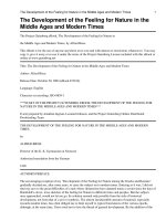
Figure 4.19: Bi-hourly ensemble UHIraw maps interpolated using data from
all stations for the entire observation period (February 2008 to Jun 2011).


117
Between 21:00 to 23:00 hrs, the highest intensities are found in the CBD, with
a warm belt stretching across the south-western coast of Singapore and a secondary
peak found over the western industrial estates. These findings are consistent with
the study conducted three decades ago by the Singapore Meteorological Services
(1986), which took measurements at 22:00 hrs (Figure 4.20). A notable feature not
present in the 1986 study is the existence of warm spots in the north and north-east,
which are expected due to rapid development of high-rise residential estates in the
past few decades.

The cool islands in the central catchment area and rural north-west also appear to have diminished in influence, possibly caused by the development of the
Bukit Timah Expressway (beginning in 1983) and the Kranji Expressway (beginning in the early 90s), along with new residential and industrial estates along the
expressway, found between the two cool zones. Another factor that may have contributed to the northward migration of the cool center in the rural north-west is the
development residential and industrial areas in the Jurong West Extension in the
early 1990s. The 1997 study by Goh and Chang (1999) found that the residential
estates in Jurong West have the highest heat island intensities among the 17 towns
sampled in Singapore.

The growth of another secondary heat island in the east is discussed in Goh
and Chang (1998), a period during which new developments in the east were completed. In the present study, large parts of the east have high UHI intensities with
the exception of a small cool spot over an airfield, noticeably different from three
decades back.


118

Figure 4.20: Isothermal maps of Singapore during the NE (top) and SW (bottom) monsoons produced with data collected over nine days between 1979 and
1981. Source: Singapore Meteorological Services (1986).


119

4.5.2

Spatial variation of ensemble mean monthly UHI across
a seasonal cycle

The spatial pattern of UHIraw also experiences seasonal variations (see Section
4.3.2). In January, during the wet and cool NE monsoon season, mean UHIraw gradients are small and both heat island and cool islands are not very developed (Figure 4.21). The highest mean intensities during this month are ∼2◦ C. In February,

UHI intensities are generally lower, with a more pronounced cool island (<0◦ C) in
the central catchment and weaker heat islands (∼1.5◦ C) in most parts of the island.

At the end of the NE monsoon in March and April, heat islands begin to grow
stronger (∼2.5◦ C) and thermal gradients are increasing. Values of mean UHIraw
continue to increase, peaking around May and June (∼3◦ C). During the south-west
monsoon, heat islands are less developed than the months before but remain strong.
Towards the end of the south-west monsoon (September and October), UHI intensities increase a little, particularly in the the heat island in the south (∼3.5◦ C). As
the north-east monsoon looms, mean intensities across the island return to lower
values, most significantly in November (∼2.5◦ C) and December (∼2◦ C).

The relative spatial differences between NE and SW monsoon are not unlike
those found in the study by Singapore Meteorological Services (1986) (Figure 4.20).
In the NE monsoon, strong heat islands are absent, with warm belts over the urban
areas. The cool islands are distinctly larger during the NE than the SW monsoon
periods. Strong heat islands are present during the SW monsoon in both studies

although some differences arise due to new urban developments discussed in the
previous section.


120

Jan

Feb

Mar

Apr

May

Jun

Captions on next page.


121

Jul

Sep

Nov

Aug

Oct

Dec

Figure 4.21: Monthly ensemble UHIraw maps using from the entire observation
period (February 2008 to July 2010) across all hours.


122

4.6

Urban effects on UHI

Land use and land cover
The land use and land cover (LULC), in terms of built-up ratio (BUP)
and vegetation ratio (VP), are calculated for the surroundings of each station
(100m and 500m radii) (Appendix B). To determine the relationship between the
above variables and the UHI-related dependent variables, linear least-square regression is used. Four types of statistical linear functions are used for curve fitting, namely, straight line (y=x), quadratic (y=x2 +x), logarithmic (y=log(x)) and
√
squared (y= x). For each pair of dependent and independent variables, the function that yields the lowest p-value is chosen as the optimal relationship. 35 stations
from S01 to S40, with the exception of stations with limited data (S16, S26, S27,
S33 and S35) are used in the regression analysis. Data used are from the entire
observation period (Feb 2008 to Jul 2011). Daytime UHI values are defined as 07:00
to 18:50 hrs and nocturnal UHI values are defined as 19:00 to 06:50 hrs.

Table 4.10, and Figures 4.22 and 4.23 show the relationships of built-up ratio at a 100 m radius (BUP100) and a 500 m radius (BUP500), vegetation ratio
at a 100 m radius (VP100) and a 500 m radius (VP500) against the dependent
variables of UHIraw and UHImax . As UHImax has daytime values filtered, daytime

mean and minimum UHImax values are irrelevant and thus left out. Comparing the
results, relationships of LULC variables with UHIraw are consistently better than
those with UHImax . This is likely due to the small size of data available for the
latter. As such, discussion will revolve around UHIraw from here on.

The LULC variables have significant relationships with nocturnal mean UHIraw ,
daytime mean UHIraw and maximum UHIraw . In particular, VP100 and VP500 explain most of the variances in nocturnal mean UHIraw (R2 > 0.6). On the other


123
hand, their predictive strengths for daytime mean UHIraw are notably weaker than
BUP100 and BUP500. Maximum UHIraw is best explained by VP500 but the other
LULC variables have relatively high R2 values too. However, none of these variables have strong relationships with minimum UHIraw , although BUP100 is weakly
correlated with it (p < 0.05).

Table 4.10: Urban variables and their relationships with dependent variables.
Observations from 35 stations for the entire observation period (Feb 2008 to Jul
2011) are used.

NM
UHIraw
DM
UHIraw
Max
UHIraw
Min
UHIraw
NM
UHImax
Max

UHImax

BUP100
y=x
0.622***
√
y= x
0.499***
y=x
0.513***
y=log(x)
0.149*
BUP100
y=x
0.576***
y=x
0.475***

BUP500
y=x
0.579***
y=x
0.385***
y=x
0.547***
y=x
0.022
BUP500
y=x
0.509***

√
y= x
0.469***

VP100
y=x
0.627***
y=x
0.290***
y=x
0.492***
y=x2 +x
0.074
VP100
y=x
0.611***
y=x
0.480***

VP500
y=x
0.677***
√
y= x
0.244**
y=x
0.608***
y=x2 +x
0.077
VP500

y=x
0.632***
y=x
0.551***

*** = p < 0.001; ** = p < 0.01; * = p < 0.05;

+

HW
y=log(x)
0.351**
√
y= x
0.243*
y=log(x)
0.321**
y=x
0.123
HW
y=log(x)
0.310**
y=log(x)
0.360**

ZH
y=log(x)
0.111
y=x
0.213**

y=log(x)
0.085
y=x
0.177*
ZH
y=log(x)
0.088
y=log(x)
0.080

SVF
y=x2 +x
0.290
y=x2 +x
0.478**
y=x2 +x
0.170
y=log(x)
0.180*
SVF
y=x2 +x
0.189
y=x2 +x
0.112

= p < 0.1;

The equations of the best performing LULC variables with strongly significant relationships (p < 0.001) are as follows:

Nocturnal mean UHIraw = −0.033 VP500 + 3.826

(4.2)

�
BUP100 − 0.238

(4.3)

Daytime mean UHIraw = 0.130

Maximum UHIraw = −0.039 VP500 + 6.562

(4.4)


●

●

2

●
●

●
●

●
●
●●

●
●

●

●

●

●
●

1
●
●
●

0

●

0

20

40

BUP100

60

80

100

●

4
●●

●

●
● ●
●●
●
●
●

3

●

●

●
●

●

●

●

●

●

●

●

●

2

●
●

●

●

●

●
●

1

●
●

0

●

●

0

20

40

60

80

VP100

100

●

1.5

●

1.0

●
●

0.5
●

0.0

●

●

●
●
●

●
●

●

●
●

●
● ●●

●

●

●●

●
●

●●

● ●

●

●

●

●
●

−0.5
−1.0
●

0

Daytime mean UHIraw(°C)

●

●

●

●

2

4

6

8

sqrt(BUP100)

●
●●

●
●

1.0

●●

●

●

●

●

●

0.5

●

●

●
●

●
●

0.0

●

●

●

●

●● ●

●
●

●

●

●

●
●

●

−0.5
−1.0
●

0

20

40

60

VP100

80

●

4

100

●●

●● ●

3

●

2

●

●
●

●

●

●
●

1
●

●
●

0

●

● ●●
● ●
●

●

●
●

●

●

●

●

●

●

●

●

0

20

40

BUP500

60

80

●

4
●

●

●
●

3

●

●●

●
●●

● ●

●

●

● ●
●

●

●

●

●

●

●

2

●

●

●

●

●

●

●

1

●
●

0

20

40

60

VP500

●

●

80

●
●

1.5
●

1.0
●
●

●

●

●

0.0

●
●
● ●

●

●

● ●

●

●

●●
●

●

●●

●

●

0.5

●

●
●

●

●

●
●

●

−0.5
−1.0
●

10

●

1.5

Nocturnal mean UHIraw(°C)

3

●

●
●

●

●●

●

●

Daytime mean UHIraw(°C)

●

Nocturnal mean UHIraw(°C)

●

4

0

Daytime mean UHIraw(°C)

Daytime mean UHIraw(°C)

Nocturnal mean UHIraw(°C)

Nocturnal mean UHIraw(°C)

124

20

40

BUP500

60

80

●

1.5

●
●
●

1.0

●

0.5

●

●
●
● ●

●●

●

●
●

●

●

●

●

●

●

●

●

●

0.0

●
●

●

●●

●
●

●

●●

−0.5
−1.0
●

2

4

6

sqrt(VP500)

8

Figure 4.22: LULC variables and their relationships with nocturnal mean
UHIraw (top) and daytime mean UHIraw (bottom). Observations from 35 stations across the entire observation period (Feb 2008 to Jun 2011) are used.
Shaded region represents the 95% confidence bands.


125
The similar slopes of the linear equations for Equations 4.2 and 4.4 (-0.033 and
-0.039 respectively) suggest that nocturnal mean UHIraw and maximum UHIraw
are influenced at similar rates by the ratio of vegetated surfaces in a 500 metre radius from each station. For every 10% increase in vegetated surface ratio, nocturnal
mean and maximum UHI decreases by 0.3 to 0.4◦ C. The base value difference (when
VP500 = 0) of just under 3◦ C is the main differentiating factor between Equations
4.2 and 4.4. As for daytime mean UHIraw , when BUP100 = 0, the base value is
-0.405◦ C. For every 25% increase in BUP100 , the daytime mean UHIraw increases
by 0.73◦ C.

●●

●

● ●
●
●
●
●
●
●
●
●

●
●

5

●

●

●●

●●

●

●

4

●

●
●
●

3

●●
●

2

0

20

40

BUP100

60

80

6
5

●

●

●●
●
●

●

●

●●

●

●

●

4

●

●
●
●

3

●●
●

2
1
40

60

VP100

80

100

●
●

●

4

●

●

●
●

3

●●
●

2
●

0

20

6
5

40

BUP500

60

80

●
●
●●
●
●

●

●
●●

●
●

●

●

●
●
●

●

●

●

●

●

●●

●

●

4

●

●
●
●

3

●

●
●

2
1

●

20

●
●

●
● ●
●●

●

●

●

●

●

●
●

●

●
●

7
●

●
● ●●
●
●
●
●
●
●
●
●

0

●

5

100

●
●

●

●
●●

6

1

●

7

●

●

Maximum UHIraw(°C)

6

1

Maximum UHIraw(°C)

7

●
●

●

Maximum UHIraw(°C)

Maximum UHIraw(°C)

7

●

20

40

VP500

60

80

Figure 4.23: LULC variables and their relationships with maximum UHIraw .
Observations from 35 stations across the entire observation period (Feb 2008 to
Jun 2011) are used. Shaded region represents the 95% confidence bands.


126
Canyon geometry
The canyon geometry factors, H/W, zH /W and SVF (see Section 3.5.2),
have been calculated for the surroundings of each station (Appendices B and D).
Among the three canyon geometry variables, H/W ratio has the highest predictive strength (p < 0.01) for nocturnal mean UHIraw and maximum UHIraw (Table
4.10). In general, zH /W ratio has the lowest predictive strength for these two dependent variables. SVF has the strongest relationship with daytime mean UHIraw
(p < 0.01). Interestingly, zH /W and SVF have weakly significant relationships with

4.5
●

4.0
●●

3.5
3.0

●
●

●

●
●

●

● ●

●

−2

Maximum UHIraw(°C)

●

●
●

●

2.5
2.0

●

●
●

●

−1

0

1

log(H/W)

2

Daytime mean UHIraw(°C)

Nocturnal mean UHIraw(°C)

minimum UHIraw (p < 0.05).

●

1.5

●
●
●

1.0

●

●

●

0.5

●●
●

0.0

● ●
●
●
●
●

●
●

●
●

●

●

●
●
●

●
●

●
●
●
●

●
●

●

−0.5
−1.0
●

0.2

0.4

SVF

0.6

0.8

7.0
●

6.5

●

●

●

●

●

6.0

●

●
●

●

5.5

●
●

●

●
●

●

● ●

5.0

●

4.5

●

−2

−1

0

log(H/W)

1

2

Figure 4.24: Canyon geometry variables and their relationships with UHI variables. Observations from 35 stations for the entire observation period (Feb 2008
to Jul 2011) are used. Note that log relationships require predictor values > 0
not present in some stations for the H/W variable, which are thus omitted in the
regression of this variable. Shaded region represents the 95% confidence bands.


127
The equations of the best performing canyon geometry variables with strong

relationships (p < 0.01) are as follows:

Nocturnal mean UHIraw = 0.293 log10 H/W + 3.426

(4.5)

Daytime mean UHIraw = 1.299 SVF − 1.885 (SVF)2 + 0.6

(4.6)

Maximum UHIraw = 0.309 log10 H/W + 6.076

(4.7)

As with LULC variables, the variable H/W best predicts both nocturnal
mean UHIraw and maximum UHIraw . The coefficient for base-10 logarithm of H/W
is similar between the two variables (0.293 and 0.309) with the main difference being the base values when log10 H/W = 0. The base values here are also similar to
those from LULC suggesting the effects of land use, land cover and urban geometry
may be linked and difficult to separate. All in all, the canyon geometry variables
do not account for UHI variance as well as the LULC variables.

A logarithmic relationship between height-width ratio and UHI intensity is
also identified by Oke (1981) when comparing H/W in city centres against their
respective UHIM AX . However, little or no studies have verified this relationship and
a past study on Singapore by Goh and Chang (1999) also questions the logarithmic
relationship. However, the present study reports a relatively better performance of
H/W in predicting night time UHI values in this study (R2 = 0.351) as compared
to the study by Goh and Chang (R2 = 0.285) which uses a median H/W across the
estate to predict heat island intensity in a straight-line function. As the H/W ratio
used in the present study focuses on the immediate proximity of the sensor, it may

be indicative of the relative importance of microscale variables.


128

Urban metabolism
In the previous discussion on QF , two possible means of QF influencing UHI
are identified. There is the spatial variation of QF dependent on the land use and
function, as well as the temporal variation due temporal differences in patterns of
anthropogenic activity (e.g. Sailor, 2011; Quah and Roth, 2012). As comprehensive
data for anthropogenic flux for each station is not available, surrogate variables are
used to identify any significant effects. Spatial variation of QF is difficult to detach
from existing urban variables such as built-up ratio and is omitted. With regards
to temporal variability, significant variations in QF within a week (weekdays vs
weekends) are identified by (Quah and Roth, 2012). If QF plays an important role
in influencing UHI in the study area, comparing weekday (Mon to Fri) and weekend
(Sat and Sun) observations would yield identifiable differences as most Singaporeans have a 5-day working week.

●
●

6

●
●
●

●

●●●

●●
●

●
●●
● ●● ●●
●
●
●
●
● ● ●
●

3
●●

●

2

●

●

●
●

●
●
●

●
●

1

●

●

Weekday max UHIraw(°C)

Weekday mean UHIraw(°C)

4

●
●
● ●
●

5

●

●
●●

4

●

●
● ●

●

●
●

3

●

●
●

2

●

1

●
●

●
●
●
●● ● ● ●
●
●

●
●
●
● ●
●
●

●
●

●

●

0

0
0

1

2

3

Weekend mean UHIraw(°C)

4

0

1

2

3

4

Weekend max UHIraw(°C)

5

6

Figure 4.25: Scatter plots of mean UHIraw (left) and maximum UHIraw (right)
during weekdays and weekends and 1:1 lines. Data are taken from all stations
for the entire observation period (Feb 2008 to Jul 2011).

Figure 4.25 shows the relationship between weekend and weekday mean


129
Table 4.11: Distribution of stations and a comparison of their maximum
UHIraw values for weekdays and weekends. Data are taken from all stations
across the entire observation period (Feb 2008 to Jul 2011). WE = weekends,
WD = weekdays.
Type
Commercial

WD UHIraw < WE UHIraw

Low-rise
residential
High-rise
residential
Mixed
Industrial
Rural/park
Coastal

S05, S32

WD UHIraw > WE UHIraw
S07, S18, S22, S24, S29,
S31, S33, S42, S44, S45, S46
S15, S19, S21

S06

S08, S14, S17, S37, S38

S20, S40
S25
S03, S10, S11, S28
S09

S13, S33, S41, S43
S02, S12, S36
S04, S23, S27, S30, S34, S39

S01

UHIraw and maximum UHIraw intensities. Paired t-test tests (N = 43) show that
while weekday and weekend mean UHIraw intensities do not have a significant relationship (t = −2.03; p > 0.01), weekday and weekend maximum UHIraw intensities
have significantly different means (t = 5.50; p < 0.001). It is postulated that commercial areas see higher UHIraw intensities during the weekdays due to increased
QF from anthropogenic activities (Chow and Roth, 2006; Quah and Roth, 2012).
For this purpose, Table 4.11 was drawn up. All of the commercial sites had higher
weekday than weekend maximum UHIraw intensities, consistent with the hypothesis. Industrial stations are also expected to have lower QF during weekends and
three of these stations (S02, S12 and S36) had higher maximum weekday UHIraw
intensities than weekend maximum UHIraw intensities. Only one industrial station
(S25) had the opposite relationship. For residential stations (both low-rise and
high-rise), three stations (S05, S06 and S32) had higher weekend maximum UHIraw
intensities than weekday maximum UHIraw intensities. However, eight other residential stations had the opposite relationship. There is almost an equal number of
stations sited in rural areas, parks and coastal areas in both categories.


130

4.7

Weather effects on monthly UHI

Earlier sections studied the variation of air temperature and consequently UHI,
given ”mean” conditions across the entire study period and filtering for weather
conditions. This section investigates the influence of synoptic weather conditions
on mean monthly UHI intensities across all stations. As we are interested in the
longer-term effects of weather, the non-filtered definition of UHI, ΔTu−r , will be
used. Due to a lack of synoptic data with high spatio-temporal resolution, monthly
data from Changi Meteorological Station will be used as a surrogate.

On a day-to-day basis, the effects of extreme weather conditions have a more
pronounced effect but it is difficult to isolate the effects of synoptic conditions on
UHI. For example, in an ideal situation, the same amount of rain has to fall at
the same intensity over both the urban and rural sites, ceteris paribus. Any asynchronous occurrence of discrete weather conditions, such as rainfall events, will
bring about artificial increases or decreases in UHI. When averaging across entire
months, relationships between weather conditions and UHI become more clear

Air temperature
Regression plots of monthly air temperature at Changi Meteorological Station against monthly mean and monthly mean maximum UHI (Figure 4.26) show
significant positive relationships (p < 0.001) with R2 values above 0.5. Based on the
regression equations, mean and maximum monthly UHI increase by 0.274◦ C and
0.411◦ C, respectively, with every degree increase in air temperature. Air temperature, however, may not be the direct factor that influences the UHI but correlated
along with other influential factors such as solar radiation and drier conditions,


131
similar to the differences between winter and summer UHI in temperate countries
(Oke, 1982).

Rainfall
Interestingly, there are no significant relationships (p > 0.1; R2 < 0.1) between total monthly rainfall, and either mean or maximum UHI intensities. A
second monthly variable, number of rain days, was also tested against mean and
maximum UHI intensities and similarly yielded no significant relationships. A possible explanation is that soil moisture (and hence thermal admittance) is a more
important variable and has a lagged relationship with rainfall events.

Wind speed
Monthly mean wind speeds have significant negative relationships with monthly
mean and maximum UHI intensities (p < 0.001 and p < 0.01 respectively), with
coefficients of determination at 0.298 and 0.414 respectively. With every ms−1 increase in wind speed, monthly mean and maximum UHI intensities are expected to
decrease by 0.284 and 0.485 ◦ C respectively. This finding is consistent with previous research showing the influence of wind on UHI intensities (e.g. Oke, 1998) and

with the study on Singapore by Chow and Roth (2006).


132

Mean UHI intensity (°C)

●

2.0
●

●

●

●

1.5

●

●
●

●
●

●

●

●

●

●

●

●

●
●

●

●

●
●

●

●
●
●

1.0

●
●

26.5

27.0

27.5

28.0

Air temperature at Changi Met Station(°C)

28.5

29.0

Mean UHI intensity (°C)

●

2.0

●

●

●

1.5

●

●

●

●
●

●
●

●

●

●

●

●

●
●
●

●

●● ●

●

●

●
●

1.0

●
●

0

100

200

300

400

Monthly rain at Changi Met Station(mm)

500

Mean UHI intensity (°C)

●

2.0
●
●

1.5

●

●

●
●

●
●

●
● ●

●

●

●

●

●
●

●●

●

●
●

●
●

●
●

1.0

●
●

1.5

2.0

2.5

Wind speed at Changi Met Station(m/s)

3.0

Figure 4.26: Regression of monthly mean UHI intensity against (top) air temperature, (middle) total monthly rainfall, and (bottom) mean wind speed. Note

that UHI intensity here is ΔTu−r . Observations from 35 stations for the entire
observation period (Feb 2008 to Jul 2011) are used. Shaded region represents
the 95% confidence bands.


Max UHI intensity (°C)

133

●

3.0

●
●

● ●
● ●

●

2.5

●

●

●

●

●

●
●
●

●
●
●

●

●

●

●
●

●

2.0

●
●

●

●

26.5

27.0

27.5

28.0

Air temperature at Changi Met Station(°C)

28.5

29.0

Max UHI intensity (°C)

●

3.0

●

●

●

●
●

●● ● ●

●

●

●

●

2.5

●

●
●

●

●
●

●
●

●

●

●

2.0
●
●

●
●

0

100

200

300

400

Monthly rain at Changi Met Station(mm)

500

Max UHI intensity (°C)

●

3.0

●
●

2.5

●● ●

●

●
●

●

●

●

●

●

●
●

●

●
●
●

●

●

●

●

●

2.0
●
●

●
●

1.5

2.0

2.5

Wind speed at Changi Met Station(m/s)

3.0

Figure 4.27: Regression of monthly maximum UHI intensity against (top) air
temperature, (middle) total monthly rainfall, and (bottom) mean wind speed.
Note that UHI intensity here is ΔTu−r . Observations from 35 stations for the entire observation period (Feb 2008 to Jul 2011) are used. Shaded region represents
the 95% confidence bands.

134

4.8

Landscape effects on UHI

As the study area is relatively small in area and located near the equator, landscape
effects studied are limited to lapse rate due to elevation and proximity from water
bodies. Table 4.12 shows the matrix of coefficients of determination (R2 ) between
the landscape factors (elevation, distance from sea and distance from large water
body) and dependent variables of UHIraw .

Table 4.12: Landscape factors and the strength of their relationship (coefficients of determination) with dependent variables. A large water body is defined
as a lake or reservoir with an area larger than 1 km2 including the sea.
Elevation
Min UHIraw
Max UHIraw
Max UHIraw(t)
hrly ens.
NM UHIraw
DM UHIraw

0.043
0.016
0.049
0.005
0.183**

Distance
from sea
0.018
0.089+
0.016

Distance from
large water body
0.025
0.000
0.058

0.056
0.007

0.000
0.106*

*** = p < 0.001; ** = p < 0.01; * = p < 0.05; + = p < 0.1;
NM = nocturnal mean; DM = daytime mean

Minimum UHIraw does not appear to be influenced by any landscape effects,
with R2 values not exceeding 0.05. The time of occurrence of maximum hourly
ensemble UHIraw and nocturnal mean UHIraw also do not show any significant relationships with landscape variables. A weakly significant (p < 0.1) relationship is
found between maximum UHIraw and distance from sea. However, this relationship account for only ∼9% of the variance. The strongest relationships are found
between elevation and daytime mean UHIraw (p < 0.01; R2 = 0.183) and distance

from large water body and daytime mean UHIraw (p < 0.05; R2 = 0.106)(Figure
4.28). UHIraw reducing with elevation is intuitive due to adiabatic cooling. For the

135
(a)
●
●

1.5

●
●
●

Daytime mean UHIraw(°C)

●

1.0

●
●
●

●

●
●

●

●

●

●

●

●
●

●

0.5

●
●

●

●

●

●

●

●

●

●

●
●

●

●

●
●

0.0

●

●

●

●

−0.5

y = 1.1 + −0.027 ⋅ x, r 2 = 0.183
●

−1.0
●

●

10

20

30

40

Elevation (m)

50

(b)
●
●

1.5

●
●

Daytime mean UHIraw(°C)

●

●

●
●
●

1.0

●
●
●

●

●

●
●
●

●

●

●

●

●

●
●

●
●
●

●
●

●

0.5

●

●●

●

●

●

0.0

●

●
●

●

−0.5

y = 0.22 + 0.00018 ⋅ x, r 2 = 0.106
●

−1.0
●

0

●

1000

2000

3000

Distance from large water body (m)

4000

Figure 4.28: Relationship between daytime mean UHIraw and (a) elevation,
and (b) distance from large water body. Observations from all stations across
the entire observation period (Feb 2008 to Jul 2011) are used. Shaded region
represents the 95% confidence bands.

latter, the relationship is also consistent with the moderating effect of the cooler
large water bodies in the day as daytime mean UHIraw decrease closer to the water

bodies.


136

Chapter 5
Summary and Conclusions
The precise definition of UHI terms used in this study, the description of instrumentation metadata and the accounting for various confounding factors such as weather
and thermal inertia are in-line with the criteria laid out by Stewart (2011). This
achieves the initial goal of having a scientifically robust UHI study. Comparison of
certain summary values suggests that stricter filtering (i.e. UHImax ) has a higher
accuracy when dealing with extreme values.
• Definition of UHI intensity following Lowry (1977) and including the known
confounding factors of landscape effect (L), weather factor (Φw ), moisture
factor (Φm ) and antecedent conditions (Φa ) : ΔT = ((Tu − Lu ) − (Tr −
Lr ))Φw Φm Φa .
• The removal of nights with antecedent weather conditions (Φa ), results in
lower UHImax than UHIraw suggesting some form of influence by unequal
antecedent conditions in UHIraw . Thus, UHImax filtering is more accurate for
reporting extreme values.
• Stricter UHImax filtering see less unexpected time of maximum UHI values
than using UHIraw filtering


137
The goal of completing an extensive monitoring exercise was achieved as observations span a period of 41 months and across 44 stations. This is the most extensive
study both spatially and temporally in Singapore to date. Results corroborate with
earlier studies and also provide new findings. From the findings of this study we can
also conclude that the UHI in Singapore exhibits strong diurnal trends linked with
time of day and strong seasonal trends linked with monsoonal seasons. Inter-annual

trending, however, does not appear to be significant.
• The previous longest study was conducted by Chow and Roth (2006), for a
period of 13 months. This is the first study to have a few years of data,
allowing for inter-annual analysis.
• Across all weather conditions without filtering, maximum air temperature

was 36.59◦ C at 15:00 hrs on March 10, 2010 (S11). Minimum air temperature

was 20.08◦ C at 06:20 hrs on 19 January 2009 (S23).
• Maximum recorded air temperature has no distinct relationship with either
mean air temperature (R2 = .0196) or minimum air temperature (R2 = .001).

However, mean air temperature and minimum air temperature have a statistically significant relationship (p < 0.01; R2 = .762).
• The highest UHIM AX (with UHImax filter) values was 6.46◦ C, measured at
22:20 hrs local time on 24th April 2009, at S22. Time of occurrence (3 hours
after sunset) and location (commercial core) are consistent with previous studies (Singapore Meteorological Services, 1986; Chow and Roth, 2006) although
magnitude is half a degree lower than what Chow and Roth (2006) found.
• Stations found in rural and vegetated areas tend to have maximum UHIraw
occurring close to sunrise.


138
• Most maximum values for both UHIraw and UHImax are found during the
April-May (Pre-SW monsoon) and July-Sept (SW monsoon) period.
• The daytime mean UHIraw intensities are similar across the study area. Small
cool islands are found in the rural north-west and the central catchment area.
Small heat islands are found in urban areas across the island. The core of
the city does not have a distinctive daytime UHI formation, possibly due to
shading by tall buildings.
• The largest daytime mean UHIraw intensity is ∼1.5◦ C and is located in the

middle of Singapore, in a large and dense low-rise residential area (S05 and
S19).
• Night-time mean UHIraw is most pronounced over the city centre and other
warm areas occur in industrial and residential zones. The night-time mean
UHIraw intensities exceed 3.5◦ C in several parts of Singapore. Steep isolines
suggest that the thermal gradient is significantly larger at night, expected due
to the different rates of cooling.
• The diurnal characteristics of the heat island changes across the year, in terms
of magnitude, standard deviation across stations, onset, peak and decline.
• Pre-SW inter-monsoon and SW monsoon periods have the highest heat island
intensities. Pre-NE inter-monsoon experiences a drop in UHI intensity and
the lowest values occur during the NE monsoon, which also experiences later
time of peak occurrence.
• Although seasonal trends are distinct, inter-annual trends do not appear to
have much influence on UHI patterns. A longer study may yield better results.
• A temporal autocorrelation analysis suggests that ΔTu−r values within four
hours are highly correlated. Over a longer period, auto-correlations around


139
the same hour of day remain largely significant (Durbin-Watson test: p <
0.001) for about 25 days.

Causal factors of UHI have been established in the study. This achieves the final
objective of this research. Several urban parameters are found to be significant
in influencing UHI-based dependent variables. Unlike synoptic weather conditions
such as air temperature and wind, landscape effects do not appear to be influential
in determining UHI magnitudes and behaviour in Singapore.
• The LULC variables have significant relationships with nocturnal mean UHIraw ,
daytime mean UHIraw and maximum UHIraw . VP100 and VP500 explain

much of the nocturnal mean UHIraw (R2 > 0.6). BUP100 and BUP500 explain much of the daytime mean UHIraw . None of the LULC variables have
strong relationships with minimum UHIraw .
• H/W ratio has the highest predictive strength (where p < 0.01) for nocturnal
mean UHIraw and maximum UHIraw (log relationships). zH /W ratio has the
lowest predictive strength. SVF has strongest relationship with daytime mean
UHIraw (p < 0.01). zH /W and SVF have weakly significant relationships with
minimum UHIraw (p < 0.05).
• Base values of regression equations of canyon geometry are similar to LULC
suggesting the effects of land-use, land cover and urban geometry are linked
and difficult to separate. Canyon geometry variables do not account for UHI
variance as well as the LULC variables.
• Weekly variability of QF has more influence over maximum UHIraw intensities
(p < 0.001) than mean UHIraw intensities. All commercial sites had higher
weekday maximum UHIraw intensities than weekend maximum UHIraw intensities. The same result applies for most industrial stations.