Complex field analysis of temporal and spatial techniques in digital holographic interferometry
Bạn đang xem bản rút gọn của tài liệu. Xem và tải ngay bản đầy đủ của tài liệu tại đây (5.09 MB, 132 trang )
COMPLEX FIELD ANALYSIS OF TEMPORAL AND
SPATIAL TECHNIQUES IN DIGITAL HOLOGRAPHIC
INTERFEROMETRY
BY
CHEN
HAO
(B. Eng)
A THESIS SUBMITTED
FOR THE DEGREE OF MASTER OF ENGINEERING
DEPARTMENT OF MECHANICAL ENGINEERING
NATIONAL UNIVERSITY OF SINGAPORE
2007
ACKNOWLEDGEMENTS
ACKNOWLEDGEMENTS
I would like to thank my supervisors A/Prof. Quan Chenggen and A/Prof.
Tay Cho Jui for their advice and guidance throughout his research. I would like to
take this opportunity to express my appreciation for their constant support and
encouragement which have ensured the completion of this study.
Special thanks to all staffs of the Experimental Mechanics Laboratory. Their
hospitality makes me enjoy my study in Singapore as an international student.
I would also like to thank my peer research students, who contribute to perfect
research atmosphere by exchanging their ideas and experience.
My thanks also extend to my family for all their support.
Last but not least, I wish to thank National University of Singapore for
providing a research scholarship which makes this study possible.
i
TABLE OF CONTENTS
TABLE OF CONTENTS
ACKNOWLEDGEMENTS
i
TABLE OF CONTENTS
ii
SUMMARY
v
NOMENCALTURE
vii
LIST OF FIGURES
ix
LIST OF TABLES
xiii
INTRODUCTION
1
1.1
Background
1
1.2
The Scope of work
6
1.3
Thesis outline
7
LITERATURE REVIEW
8
Foundations of holography
8
2.1.1
Hologram recording
8
2.1.2
Optical reconstruction
10
2.2
Holographic interferometry (HI)
11
2.3
Digital holography (DH)
14
Types of digital holography
15
CHAPTER 1
CHAPTER 2
2.1
2.3.1
2.3.1.1
General Principles
15
2.3.1.2
Reconstruction by the Fresnel Approximation
16
2.3.1.3
Digital Fourier holography
18
2.3.1.4
Phase shifting digital holography
19
2.4
Digital holographic interferometry
22
2.5
Phase unwrapping
22
2.5.1
Spatial Phase Unwrapping
23
2.5.2
Temporal Phase Unwrapping
24
2.6
Temporal phase unwrapping of digital holograms
24
2.7
Short time Fourier transform (STFT)
26
ii
TABLE OF CONTENTS
2.7.1
An introduction to STFT
26
2.7.2
STFT in optical metrology
27
2.7.2.1
Filtering by STFT
28
2.7.2.1
Ridges by STFT
28
THEORY OF COMPLEX FIELD ANALYSIS
30
3.1
D.C.-term of the Fresnel transform
30
3.2
Spatial frequency requirements
34
3.3
Deformation measurement by HI
39
3.4
Shape measurement by HI
41
3.5
Temporal phase unwrapping algorithm
42
3.6
Complex field analysis
42
3.7
Temporal phase retrieval from complex field
41
3.7.1
Temporal Fourier transform
41
3.7.2
Temporal STFT analysis
47
CHAPTER 3
3.7.2.1
Temporal filtering by STFT
47
3.7.2.2
Temporal phase extraction from a ridge
48
3.7.2.3
Window Selection
51
3.7.3
Spatial phase retrieval from a complex field
3.7.4
Combination of temporal phase retrieval and spatial
phase retrieval
54
57
DEVELOPMENT OF EXPERIMENTATION
58
Equipment for dynamic measurement
58
4.1.1
High speed camera
58
4.1.2
PZT translation stage
59
4.1.3
Stepper motor travel linear stage
60
4.1.4
Specimens
61
Equipment for Static Measurement
63
4.2.1
High resolution digital still camera
63
4.2.2
Specimen
63
Experimental setup
64
Multi-illumination method
64
CHAPTER 4
4.1
4.2
4.3
4.3.1
iii
TABLE OF CONTENTS
4.3.2
Measurement of continuously deforming object
64
RESULTS AND DISCUSSION
67
5.1
D.C-term removal
68
5.2
Spatial CP method
71
5.3
Temporal CP method in dynamic measurement
75
5.3.1
Surface profiling on an object with step change
75
5.3.2
Measurements on continuously deforming object
83
5.3.3
A comparison of three temporal CP algorithms
89
CONCLUSIONS AND FUTURE WORK
97
6.1
Conclusions
97
6.2
Future work
99
CHAPTER 5
CHAPTER 6
REFERENCES
101
APPENDICES
108
A.
SHORT TIME FOURIER TRANSFORM RIDGES
108
B.
C++ SOURCE CODE FOR TEMPORAL RIDGE
112
ALGORITHM
C.
LIST OF PUBLICATIONS DURING M.ENG PERIOD
118
iv
SUMMARY
SUMMARY
In this thesis, a novel concept of complex phasor method to process the digital
holographic interference phase maps in complex field is proposed. Based on this
concept, three temporal phase retrieval algorithms and one spatial retrieval approach
are developed. Temporal complex phasor method is highly immune to noise and
allows accurate measurement of dynamic object. A series of digital holograms is
recorded by a high-speed camera during the continuously illumination changing or
deformation process of the tested specimen. Each digital hologram is numerically
reconstructed in the computer instead of optically, thus a sequence of complex-valued
interference phase maps are obtained by the proposed concept. The complex phasor
variation of each pixel is measured and analyzed along the time axis.
The first temporal complex phasor algorithm based on Fourier transform is
specially developed for dynamic measurement in which the phase is linearly dependent
on time. By transforming the sequence of complex phasors into frequency domain, the
peak corresponding to the rate of phase changing is readily picked up. The algorithm
works quite well even when the data is highly noise-corrupted. But the requirement on
linear changing phase constrains its real application.
The short time Fourier transform (STFT) which is highly adaptive to exponential
field is employed to develop the second and third algorithms. The second algorithm
also transforms the sequence of complex phasors into frequency domain, and discards
coefficients whose amplitude is lower than preset threshold. The filtered coefficients
are inverse transformed. Due to the local transformation, bad data has no effect on data
beyond the window width, which is a great improvement over the global transform, e.g.
v
SUMMARY
Fourier transform. Another advantage of STFT is that it is able to tell when or where
certain frequency components exist. The instantaneous frequency retrieval of the
complex phasor variation of a pixel is therefore possible by the maximum modulus-the
ridge-of a STFT coefficient. The continuous interference phase is then obtained by
integration. It is possible to calculate the first derivative of the measured physical
quantity using this method, e.g. velocity in deformation measurement.
To demonstrate the validity of proposed temporal and spatial methods, two
dynamic experiments and one static experiment are conducted: the profiling of surface
with height step, instantaneous velocity and deformation measurement of continuously
deforming object and deformation measurement of an aluminum plate. The commonly
used method of directly processing phase values in digital holographic interferometry
is employed for comparison. It is observed that the proposed methods give a better
performance.
The complex phasor processing as proposed in this study demonstrates a high
potential for robust processing of continuous sequence of images. The study on
different temporal phase analysis techniques will broaden the applications in optical,
nondestructive testing area, and offer more precise results and bring forward a wealth
of possible research directions.
vi
NOMENCLATURE
NOMENCLATURE
E
Electrical field form of light waves
a
Real of amplitude of light wave
ϕ
The phase of light wave
I
Intensity of light wave
h
Amplitude transmission
Δϕ
Interference phase
Γ
Complex field of light wave
d
Distance between object and hologram plane
Re
Real part of a complex function
Im
Imaginary part of a complex function
Δξ
Pixel size along x direction
Δη
Pixel size along y direction
f max
Maximum spatial frequency
θ max
Maximum angle between object and reference wave
δ
Optical path length difference
Sf
Short time Fourier transform
Ps f
Spectrogram of short time Fourier transform
ξ
Spatial frequency along x direction
η
Spatial frequency along y direction
A
Complex field by conjugate multiplication
vii
NOMENCLATURE
Δϕ w
ℑ
Wrapped interference phase
Fourier transform
Δϕ ’
First derivative of interference phase
Tx
Time width of signal
Bx
Frequency domain bandwidth
gTBP
Optimized window
viii
LIST OF FIGURES
LIST OF FIGURES
Fig. 2.1
Schematic layout of the hologram recording setup
Fig. 2.2
Schematic layout of optical reconstruction
10
Fig. 2.3
Recording of a double exposure hologram
12
Fig. 2.4
Reconstruction
13
Fig. 2.5
Coordinate system for numerical hologram reconstruction
15
Fig. 2.6
Digital lensless Fourier holography
19
Fig. 2.7
Phase shifting digital holography
20
Fig. 2.8
Procedure for temporal phase unwrapping of digital holograms
(Pedrini et al., 2003)
25
Phase retrieval from phase-shifted fringes: (a) one of four phaseshifted fringe patterns; (b) phase by phase-shifting technique and
(c) phase by WFR (Qian, 2007)
29
Fig. 2.10 WFR for strain extraction: (a) Original moiré fringe pattern; (b)
strain contour in x direction using moiré of moiré technique and
(c) strain field by WFR (Qian, 2007)
29
Fig. 2.9
Fig. 3.1
9
A reconstructed intensity distribution by Fresnel transform
without clipping
30
Fig. 3.2
Digital lensless Fourier holography
34
Fig. 3.3
Spatial frequency spectra of an off-axis holography
36
Fig. 3.4
Geometry for recording an off-axis digital Fresnel hologram
37
Fig. 3.5
Geometry for recording an off-axis digital lensless Fourier
hologram
38
Schematic illustration of the angle between the object wave and
reference wave in digital lensless Fourier holography setup
(Wagner et al., 1999)
38
Sensitivity vector for digital
measurement of displacement
40
Fig. 3.6
Fig. 3.7
holographic
interferometric
ix
LIST OF FIGURES
Fig. 3.8
Two-illumination point contouring
41
Fig. 3.9
A linearly changing phase
45
Fig. 3.10 The spectrum of a complex phasor with linearly changing phase
45
Fig. 3.11 Comparison of STFT resolution: (a) a better time solution; (b) a
better frequency solution
52
Fig. 3.12 Spectrograms with different window width: (a) 25 ms; (b) 125
ms; (c) 375 ms; (d) 1000 ms
54
Fig. 3.13 Unfiltered interference phase distribution
55
Fig. 3.14 (a) Effect of filtering a phasor image; (b) effect of sine/cosine
transformation
56
Fig. 3.15 Flow chart of (a) conventional method (b) proposed method
57
Fig. 4.1
Kodak Motion Corder Analyzer, Monochrome Model SR-Ultra
59
Fig. 4.2
PZT translation stage (Piezosystem Jena, PX 300 CAP) and its
controller
60
Fig. 4.3
Newport UTM 150 mm mid-range travel steel linear stage
60
Fig. 4.4
Melles Griot 17 MDU 002 NanoStep Motor Controller
61
Fig. 4.5
(a) Dimension of a step-change object; (b) top view of the
specimen with step-change.
61
(a) A cantilever beam and its loading device; (b) Schematic
description of loading process and inspected area
62
Fig. 4.7
Pulnix TM-1402
63
Fig. 4.8
A circular plate centered loaded
63
Fig. 4.9
Optical arrangement for profile measurement using multiillumination-point method
65
Fig. 4.6
Fig. 4.10 Digital holographic setup for dynamic deformation measurement
66
Fig. 5.1
A typical digital hologram
68
Fig. 5.2
Intensity display of a reconstruction with D.C.-term eliminated
69
Fig. 5.3
Intensity distribution display of reconstruction: (a) with average
x
LIST OF FIGURES
value subtraction only; (b) with high-pass filter only
69
(a) digital hologram in digital lensless Fourier holography; (b) Its
corresponding intensity display of reconstruction with D.C.-term
eliminated
70
Intensity display of reconstruction: (a) with average value
subtraction; (b) with high-pass filter only
70
Fig. 5.6
Process flow of digital holographic interferometry
72
Fig. 5.7
Spatial phase unwrapping
73
Fig. 5.8
Spatial phase retrieval by CP method
74
Fig. 5.9
Digital hologram in surface profiling experiment (particles are
highlighted by circles)
75
Fig. 5.4
Fig. 5.5
Fig. 5.10 Reconstruction of Figure 5.9
76
Fig. 5.11 DPS method
77
Fig. 5.12
(a) Wrapped phase for a given point; (b) Unwrapped phase for a
given point
79
Fig. 5.13
(a) Unwrapped phase; (b) corresponding 3D plot
79
Fig. 5.14
(a) Phase variation of a pixel; (b) intensity variation of a pixel
80
Fig. 5.15 Frequency spectrum of a pixel
80
Fig. 5.16 Unwrapped phase by integration
80
Fig. 5.17 Results calculated by temporal Fourier transform algorithm: (a)
unwrapped phase; (b) 3D plot
81
Fig. 5.18 Result for a pixel by temporal STFT filtering: (a) Wrapped phase;
(b) Unwrapped phase
82
Fig. 5.19 Results calculated temporal STFT filtering algorithm: (a)
unwrapped phase; (b) 3D plot
82
Fig. 5.20 Triangular wave by PZT stage
84
Fig. 5.21 Digital hologram and its intensity display of reconstruction
84
Fig. 5.22 Interference phase variations with time
85
Fig. 5.23 Schematic description of temporal phase unwrapping of digital
xi
LIST OF FIGURES
holograms
86
Fig. 5.24 A typical interference phase pattern of the cantilever beam
86
Fig. 5.25 Unwrapped phase by DPS method
86
Fig. 5.26 (a) Instantaneous velocity of point B using numerical
differentiation of unwrapped phase difference; (b) Instantaneous
velocity of points A, B and C by proposed ridge algorithm
88
Fig. 5.27 Flow chart of instantaneous velocity calculation using CP method
90
Fig. 5.28 2D distribution and 3D plots of instantaneous velocity at various
instants
91
Fig. 5.29 Displacement of point B: (a) by temporal phase unwrapping of
wrapped phase difference using DPS method; (b) by temporal
phase unwrapping of wrapped phase difference from t = 0.4s to t
= 0.8s using DPS method; (c) by integration of instantaneous
velocity using CP method; (d) by integration of instantaneous
velocity from t = 0.4s to t = 0.8s using CP method
93
Fig. 5.30 3D plot of displacement distribution at various instants. (a), (c),
(e) by integration of instantaneous velocity using CP method; (b),
(d), (f) by temporal phase unwrapping using DPS method
94
xii
LIST OF TABLES
LIST OF TABLES
Table 5.1
A comparison of different temporal algorithms from CP concept
96
xiii
CHAPTER ONE
INTRODUCTION
CHAPTER ONE
INTRODUCTION
1.1
Background
Dennis Gabor (1948) invented holography as a lensless means for image formation by
reconstructed wavefronts. He created the word holography from the Greek words
‘holo’ meaning whole and ‘graphein’ meaning to write. It is a clever method of
combining interference and diffraction for recording the reconstructing the whole
information contained in an optical wavefront, namely, amplitude and phase, not just
intensity as conventional photography does. A wavefield scattered from the object and
a reference wave interferes at the surface of recording material, and the interference
pattern is photographically or otherwise recorded. The information about the whole
three-dimensional wave field is coded in form of interference stripes usually not
visible for the human eye due to the high spatial frequencies. By illuminating the
hologram with the reference wave again, the object wave can be reconstructed with all
effects of perspective and depth of focus.
Besides the amazing display of three-dimensional scenes, holography has found
numerous applications due to its unique features. One major application is Holographic
Interferometry (HI), discovered by Stetson (1965) in the late sixties of last century.
Two or more wave fields are compared interferometrically, with at least one of them is
holographically recorded and reconstructed. Traditional interferometry has the most
stringent limitation that the object under investigation be optically smooth, however,
HI removes such a limitation. Therefore, numerous papers indicating new general
1
CHAPTER ONE
INTRODUCTION
theories and applications were published following Stetsons’ publication. Thus HI not
only preserves the advantages of interferometric measurement, such as high sensitivity
and non-contacting field view, but also extends to the investigation of numerous
materials, components and systems previously impossible to measure by classical
optical method. The measurement of the changes of phase of the wavefield and thus
the change of any physical quantity that affects the phase are made possible by such a
technique. Applications ranged from the first measurement of vibration modes (Powell
and Stetson, 1965), over deformation measurement (Haines and Hilderbrand, 1966a),
(1966b), contour measurement (Haines and Hilderbrand, 1965), (Heflinger, 1969), to
the determination of refractive index changes (Horman, 1965), (Sweeney and Vest,
1973).
The results from HI are usually in the form of fringe patterns which can be
interpreted in a first approximation as contour lines of the amplitude of the change of
the measured quantity. For example, a locally higher deformation results in a locally
higher fringe density. Besides this qualitative evaluation expert interpretation is needed
to convert these fringes into desired information. In early days, fringes were manually
counted, later on interference patterns were recorded by video cameras (nowadays
CCD or CMOS cameras) for digitization and quantization. Interference phases are then
calculated from those stored interferograms, with initially developed algorithms
resembling the former fringe counting. The introduction of the phase shifting methods
of classic interferometric metrology into HI was a big step forward, making it possible
to measure the interference phase between the fringe intensity maxima and minima and
at the same time resolving the sign ambiguity. However, extra experimental efforts
were required for the increased accuracy. Fourier transform evaluation (Kreris, 1986)
2
CHAPTER ONE
INTRODUCTION
is an alternative without the need for generating several phase shifted interferograms
and without the need to introduce a carrier (Taketa et al., 1982).
While holographic interferograms were successfully evaluated by computer, the
fabrication of the interference pattern was still a clumsy work. The wet chemical
processing of the photographic plates, photothermoplastic film, photorefractive
crystals, and other recording media all had their inherent drawbacks. With the
development of computer technology, it was possible to transfer either the recording
process or reconstruction process into the computer. Such an endeavor led to the first
resolution: Computer Generated Holography (Lee, 1978), which generates holograms
by numerical method. Afterwards these computer generated holograms are
reconstructed optically.
Goodman and Lawrence (1967) proposed numerical hologram reconstruction
and later followed by Yaroslavski et al. (1972). They sampled optically enlarged parts
of in-line and Fourier holograms recorded on a photographic plate and reconstructed
these digitized conventional holograms. Onural and Scott (1987, 1992) improved the
reconstruction algorithm and used this approach for particle measurement.
Direct recording of Fresnel holograms with CCD by Schnars (1994) was a
significant step forward, which enables full digital recording and processing of
holograms, without the need of photographic recording as an intermediate step. Later
on the term Digital Holography (DH) was accepted in the optical metrology
community for this method. Although it is already a known fact that numerically the
complex wave field can be reconstructed by digital holograms, previous experiments
(Goodman and Lawrence, 1967) (Yaroslavski et al, 1972) concentrated only on
intensity distribution. It is the realization of the potential of the digitally reconstructed
3
CHAPTER ONE
INTRODUCTION
phase distribution that led to digital holographic interferometry (Schnars, 1994). The
phases of stored wave fields can be accessed directly once the reconstruction is done
using digitally recorded holograms, without any need for generating phase-shifted
interferograms. In addition, other techniques of interferometric optical metrology, such
as shearography or speckle photography, can be derived numerically from digital
holography. Sharing the advantages of conventional optical holographic interferometry,
DH also has its own distinguished features:
z
No such strict requirements as conventional holography on vibration and
mechanical stability during recording, for CCD sensors have much higher
sensitivity within the working wavelength than that of photographic recording
media.
z
Reconstruction process is done by computers, no need for time-consuming wet
chemical processing and a reconstruction setup.
z
Direct phase accessibility. High quality interference phase distributions are
available easily by simply subtraction between phases of different states.
Therefore, avoiding processing of often noise disturbed intensity fringe patterns.
z
Complete description of wavefield, not only intensity but also phase is available.
Thus a more flexible way to simulate physical procedures with numerical
algorithms. What is more, powerful image processing algorithms can be used for
better reconstructed results.
Digital holography (DH) is much more than a simple extension of conventional
optical holography to digital version. It offers great potentials for non-destructive
measurement and testing as well as 3D visualization. Employing CCD sensors as
recording media, DH is able to digitalize and quantize the optical information of
holograms. The reconstruction and metrological evaluations are all accomplished by
4
CHAPTER ONE
INTRODUCTION
computers with corresponding numerical algorithms. It simplifies both the system
configuration and evaluation procedure for phase determination, which requires much
more efforts, both experimentally and mathematically. Digital holography can now be
a more competing and promising technique for interferometric measurement in
industrial applications, which are unimaginable for the traditional optical holography.
In experimental mechanics, high precision 3D displacement measurement of
object subject to impact loading and vibration is an area of great interest and is one of
the most appealing applications of DH. Those displacement results can later be used to
access engineering parameters such as strain, vibration amplitude and structural energy
flow. Only a single hologram needs to be recorded in one state and the transient
deformation field can be obtained quite easily by comparing wavefronts of different
states interferometrically. In addition, there is no need at all for the employment of
troublesome phase-shifting (Huntley et al., 1999) or a temporal carrier (Fu et al., 2005)
to determine the phase unambiguously. By employing a pulsed laser, fast dynamic
displacements can be recorded quite easily, provided that each pulse effectively freezes
the object movement. Such a combination of DH and a pulsed ruby laser has been
reported for: vibration measurements (Pedrini et al., 1997), shape measurements
(Pedrini et al., 1999), defect recognition (Schedin et al., 2001) and dynamic
measurements of rotating objects (Perez-lopez, 2001). However, this technique has its
own limitation. An experiment has to be repeated several times before the evolution of
the transient deformation can be obtained, each time with a different delay. Problems
will arise when an experiment is difficult to repeat. Due to the rapid development of
CCD and CMOS cameras speed, it is now possible to record speckle patterns with
rates exceeding 10,000 frames per second. Therefore, one solution to those problems is
to record a sequence of holograms during the whole process (Pedrini, 2003).
5
CHAPTER ONE
INTRODUCTION
The quantitative evaluation of the resulting fringe pattern is usually done by
carrying out spatial phase unwrapping. However, it suffers an inherent drawback that
absolute phase values are not available. Phase value relative to some other point is
what it all can achieve. In addition, large phase errors will be generated if the pixels of
the wrapped interference phase map are not well modulated. An alternative is the one
dimensional approach to unwrap along the time axis was proposed by Huntley (1993).
Each pixel of the camera acts as an independent sensor and the phase unwrapping is
done for each pixel in the time domain. Such kind of method is particularly useful
when processing speckle patterns, and can avoid the spatial prorogation of phase errors.
In addition, temporal phase unwrapping allows absolute phase value to be obtained,
which is impossible by spatial phase unwrapping.
1.2 The Scope of work
The scope of this dissertation work is focused on temporal phase retrieval techniques
combined with digital holographic interferometry and applying them for dynamic
measurement. Specifically, (1) Study the mechanisms and properties of digital
holography with emphasis on dynamic measurement; (2) Propose a novel complex
field processing method; (3) Develop three temporal phase retrieval algorithms using
powerful time-frequency tools based on the proposed method; (4) Compare spatial
filtering techniques using the proposed method with commonly used ones; (5) Verify
those proposed methods, algorithms and techniques with different digital holographic
interferometric experiments.
1.3 Thesis outline
An outline of the thesis is as follows:
6
CHAPTER ONE
INTRODUCTION
Chapter 1 provides an introduction of this dissertation.
Chapter 2 reviews the foundations of optical and digital holography. In digital
holographic interferometry, the basis of the two-illumination-point method for surface
profiling and deformation measurement are discussed. This chapter also discusses the
advantage of digital holographic interferometry’s application to dynamic measurement.
Chapter 3 presents the theory of the proposed complex phasor method, under
which the temporal Fourier analysis, temporal STFT filtering, temporal ridge
algorithm are developed.
Chapter 4 describes the practical aspects of a dynamic phase measurement. The
setups are described.
Chapter 5 compares the results obtained by the conventional and proposed
methods. The advantages, disadvantages and accuracy of the proposed methods are
analyzed in detail.
Chapter 6 summarizes this project work and shows potential development on
dynamic measurements.
7
CHAPTER TWO
LITERATURE REVIEW
CHAPTER TWO
LITERATURE REVIEW
2.1 Foundations of holography
2.1.1
Hologram recording
An optical setup composed of a light source (laser), mirrors and lenses to guide beam
and a recording device, e. g. a photographic plate is usually used to record holograms.
A typical setup (Schnars, 2005) is shown in Figure 2.1. A laser beam with sufficient
coherence length is split into two parts by a beam splitter. One part of the wave
illuminates the object, scattered and reflected to the recording medium. The other one
acting as the reference wave illuminates the light sensitive medium directly. Both
waves interfere. The resulting interference pattern is recorded and chemically
developed.
The complex amplitude of the object wave is described by
EO ( x, y ) = aO ( x, y ) exp ⎡⎣iϕO ( x, y ) ⎤⎦
(2.1)
with real amplitude aO and phase ϕ o .
ER ( x, y ) = aR ( x, y ) exp ⎡⎣iϕ R ( x, y ) ⎤⎦
(2.2)
is the complex amplitude of the reference wave with real amplitude aR and phase ϕ R .
8
CHAPTER TWO
LITERATURE REVIEW
Mirror
Laser
Beam
Splitter
Mirror
lens
Mirror
lens
Object
Hologram
Figure 2.1 Schematic layout of the hologram recording setup
Both waves interfere at the surface of the recording medium. The intensity is
given as
I ( x, y ) = EO ( x, y ) + ER ( x, y )
2
= ⎣⎡ EO ( x, y ) + ER ( x, y ) ⎤⎦ ⎡⎣ EO ( x, y ) + ER ( x, y ) ⎤⎦
*
(2.3)
= aO2 ( x, y ) + aR2 ( x, y ) + EO ( x, y ) ER* ( x, y ) + EO* ( x, y ) ER ( x, y )
The amplitude transmission h ( x, y ) of the developed photographic plated is
proportional to I ( x, y ) :
h ( x, y ) = h0 + βτ I ( x, y )
(2.4)
9
CHAPTER TWO
LITERATURE REVIEW
The constant β is the slope of the amplitude transmittance versus exposure
characteristic of the light sensitive material. τ is the exposure time and h0 is the
amplitude transmission of the unexposed plate.
2.1.2
Optical reconstruction
The developed photographic plate is illuminated by the reference wave ER , as shown
in Figure 2.2, for optical reconstruction of the object wave. This gives a modulation of
the reference wave by the transmission h ( x, y ) :
Mirror
Laser
Beam
Splitter
Mirror
lens
Stop
Reconstructed Image
Hologram
Figure 2.2 Schematic layout of optical reconstruction
E R ( x, y ) h ( x, y ) =
(
)
⎡ h0 + βτ aR2 + aO2 ⎤ ER ( x, y ) + βτ aR2 EO ( x, y ) + βτ ER2 ( x, y ) EO∗ ( x, y )
⎣
⎦
(2.5)
10
CHAPTER TWO
LITERATURE REVIEW
The first term on the right side of the equation is the zero diffraction order, it is
just the reference wave multiplied with the mean transmittance. The second term is the
reconstructed object wave, forming the virtual image. The factor before it only
influences the brightness of the image. The third term produces a distorted real image
of the object.
2.2 Holographic interferometry (HI)
By holographic recording and reconstruction of a wave field, it is possible to compare
such a wave field interferometrically either with a wave field scattered directly by the
object, or with another holographically reconstructed wave field. HI is defined as the
interferometric comparison of two or more wave fields, at least one of which is
holographically reconstructed (Vest, 1979). HI is a non-contact, non-destructive
method with very high sensitivity. The resolution is able to reach up to one hundredth
of a wavelength.
Only slight differences between the wave fields to be compared by holographic
interferometry are allowed:
1. The same microstructure of object is demanded;
2. The geometry for all wave fields to be compared must be the same;
3. The wavelength and coherence for optical laser radiation used must be stable
enough;
4. The change of the object to be measured should be in a small range.
In double exposure method of HI, two wave fields scattered from the same
object in two different states are recorded consecutively by the same recording media
11