Computational methods for a phase field model of grain growth kinetics

COMPUTATIONAL METHODS FOR A
PHASE-FIELD MODEL OF GRAIN GROWTH
KINETICS

BIPIN KUMAR
(M.Sc., IIT Kanpur, India)

A THESIS SUBMITTED
FOR THE DEGREE OF MASTER OF SCIENCE

DEPARTMENT OF MATHEMATICS
NATIONAL UNIVERSITY OF SINGAPORE


Acknowledgments
I warmly express heartfelt gratitude and sincere appreciations to my supervisor Dr.
Lin Ping for his guidance full with patient, stimulating ideas and invaluable advice
throughout my study period in NUS. Without his supervisions, even the very first
step was not possible. It has been my pleasure being his research student.
I would like to express my sincere thanks to Dr. B.S.V. Patnaik for all his help and
guidance.
Special thanks are very much due to Dr. Shashi Bhushan (DNV), Venkateswarlu,
Zacharry Harrish, Dr. Ram Singh Rana (A*Star) and Dr. Sanjiv Yadav (Chemistry). On my mind, the proximity and moral support, I had from them, has put
indelible print of my memorable stay in Singapore.
I would next, like to thank to my officemates Jinghui, David, Chen Yidi, Wu Lei,
and Xu Ying for their assistance. Talks held with them will always remain in my
thoughts. Discussion held with Shapeev Alexander are duly acknowledged. I would
like to express my sincere feelings to my house mates Yogesh, Raju, Mohan, Ved
and my friends Sunil, Kaushal Pandey, Jan Frode Stene, Sulakshana, Khaing Mawoo Toee and Mrs Desai.
Finally, I would like to thank my parents and siblings. Without their continuous
encouragement and support, nothing would have been possible for me.

i


ii
Last but the most important feelings for Ms Preeti, who has accepted to knot with
me forever.
I feel lack of words to acknowledge Him who has provided me with unlimited potential but with limited capabilities. I bow my head to Him!!


Contents
1 Introduction
1.1

1.2

1

Motivation and Objectives: . . . . . . . . . . . . . . . . . . . . . . . .

2

1.1.1

Motivation: . . . . . . . . . . . . . . . . . . . . . . . . . . . .

2

1.1.2

Objectives: . . . . . . . . . . . . . . . . . . . . . . . . . . . .

3

Organization of this thesis: . . . . . . . . . . . . . . . . . . . . . . . .

3

2 Material Science and Simulations

5

2.1

What are Materials? . . . . . . . . . . . . . . . . . . . . . . . . . . .

5

2.2

Role of Computational Materials Science: . . . . . . . . . . . . . . . .

6

2.3

Relevance of Simulating Microstructural Evolutions: . . . . . . . . . .

7

2.4

Phase Field Model: . . . . . . . . . . . . . . . . . . . . . . . . . . . .

9

2.5

2.4.1

What is an Interface?

. . . . . . . . . . . . . . . . . . . . . . 10

2.4.2

Sharp Interface: . . . . . . . . . . . . . . . . . . . . . . . . . . 10

2.4.3

Diffuse Interface: . . . . . . . . . . . . . . . . . . . . . . . . . 11

Application of Phase Field Methods: . . . . . . . . . . . . . . . . . . 12

3 Theory and Model Description
3.1

14

Local Free Energy: . . . . . . . . . . . . . . . . . . . . . . . . . . . . 15

iii


iv

CONTENTS
3.2

Need for advanced numerical approaches: . . . . . . . . . . . . . . . . 19

4 Computational Algorithms

21

4.1

Finite Difference Approach (Explicit):

. . . . . . . . . . . . . . . . . 22

4.2

Finite Difference Approach (Semi Implicit):

4.3

Operator Splitting Method: . . . . . . . . . . . . . . . . . . . . . . . 26

. . . . . . . . . . . . . . 24

4.3.1

Exact Solution of 3rd Degree Polynomial Equation: . . . . . . 27

4.3.2

Discussion of Solution: . . . . . . . . . . . . . . . . . . . . . . 27

4.4

Active Parameter Tracking Algorithm: . . . . . . . . . . . . . . . . . 31

4.5

Finite Element Approach: . . . . . . . . . . . . . . . . . . . . . . . . 33

4.6

On the Implementation of Periodic Boundary Conditions: . . . . . . . 38

4.7

On Solving Large-Scale System of Equations: . . . . . . . . . . . . . . 39
4.7.1

Format for Sparse Matrix: . . . . . . . . . . . . . . . . . . . . 41

4.7.2

Sparse Matrix-Vector Multiplication in CSR Format: . . . . . 42

5 Results and Discussion

43

5.1

Finite Difference Method (Explicit): . . . . . . . . . . . . . . . . . . . 43

5.2

FD with Operator Splitting Method: . . . . . . . . . . . . . . . . . . 48
5.2.1

Operator Splitting: Case 1 . . . . . . . . . . . . . . . . . . . . 50

5.2.2

Operator Splitting: Case 2 . . . . . . . . . . . . . . . . . . . . 52

5.2.3

Operator Splitting: Case 3 . . . . . . . . . . . . . . . . . . . . 52

5.3

AIA-PT Method: . . . . . . . . . . . . . . . . . . . . . . . . . . . . . 54

5.4

Result Comparison and Discussion: . . . . . . . . . . . . . . . . . . . 54
5.4.1

Comparison of Result with other Researcher’s Results: . . . . 56

6 Conclusions and Suggestions for Future Work

65


CONTENTS

v

6.1

Conclusions: . . . . . . . . . . . . . . . . . . . . . . . . . . . . . . . . 65

6.2

Suggestions for Future Work: . . . . . . . . . . . . . . . . . . . . . . 66


Abstract
Computational Materials science is fast catching up as an attractive and complementary approach to designing novel materials. An apriori understanding of micro
structures and its linkage to material properties is possible through the use of workable models. In this thesis, we explore a variety of computational algorithms for
solving partial differential equations that govern the kinetics of grain growth. To
start with, we employ the emerging phase-field approach to model the micro structural evolutions.
To start with, we have to design the appropriate energy functional. Then, solve the
Allen-Cahn equations or the Complex Ginzhburg Landau equations (CGLE).

Following computational schemes are devised for the phase-field equations:

(i) Solve the equations by Finite difference method with a simple explicit time
marching scheme (This is the most popular approach)

(ii) Solve the Allen-Cahn equations using operator splitting method, where the
equation is divided into a Poisson part and a cubic equation. (Note that, the cubic
equation has an exact solution).

vi


CONTENTS

vii

(iii) A simple observation that only the interfaces have more than one active
phase-field variables at every grid point was successfully exploited by devising an
active and implicitly adaptive parameter tracking (AIA-PT) approach.

(iv) Solve the equations by Combing the two ideas of operator splitting and
AIA-PT.


List of Figures
2.1

Demonstration of multi-scale modeling for the design of radiation
resistant material : Ghoniem et al [26] . . . . . . . . . . . . . . . . .

8

2.2

Typical image of grains [27] . . . . . . . . . . . . . . . . . . . . . . .

9

3.1

Representation of Orientation field variable φ . . . . . . . . . . . . . 14

4.1

Discretization of Laplacian . . . . . . . . . . . . . . . . . . . . . . . . 23

4.2

CSR format of a sparse matrix

5.1

Temporal evolution of microstructure for FDM(explicit) for Q=48 . . 45

5.2

Temporal evolution of microstructure for FDM(explicit) for Q=60. . . 46

5.3

Temporal evolution of microstructure for FDM (explicit) scheme for

. . . . . . . . . . . . . . . . . . . . . 42

Q=36 . . . . . . . . . . . . . . . . . . . . . . . . . . . . . . . . . . . 47
5.4

The average grain area and total time taken as function of time for
FDM (explicit). . . . . . . . . . . . . . . . . . . . . . . . . . . . . . . 48

5.5

Temporal evolution of microstructure for FDM (explicit) scheme for
Q=48 . . . . . . . . . . . . . . . . . . . . . . . . . . . . . . . . . . . 49

5.6

The average grain area and total time taken as function of time for
FDM (explicit). . . . . . . . . . . . . . . . . . . . . . . . . . . . . . . 50

viii


ix

LIST OF FIGURES
5.7

Temporal evolution of microstructure for FDM (explicit) scheme for
Q=48 . . . . . . . . . . . . . . . . . . . . . . . . . . . . . . . . . . . 51

5.8

Temporal evolution of microstructure for operator splitting case 1 for
Q=36. . . . . . . . . . . . . . . . . . . . . . . . . . . . . . . . . . . . 53

5.9

The average grain area and total time taken as function of time for
operator splitting case 1. . . . . . . . . . . . . . . . . . . . . . . . . . 54

5.10 Temporal evolution of microstructure for operator splitting case 1 for
Q=48 . . . . . . . . . . . . . . . . . . . . . . . . . . . . . . . . . . . 55
5.11 The average grain area and total time taken as function of time for
FDM (explicit). . . . . . . . . . . . . . . . . . . . . . . . . . . . . . . 56
5.12 Temporal evolution of microstructure for operator splitting case 2 for
Q=36. . . . . . . . . . . . . . . . . . . . . . . . . . . . . . . . . . . . 57
5.13 The average grain area and total time taken as function of time for
operator splitting case 2. . . . . . . . . . . . . . . . . . . . . . . . . . 58
5.14 Temporal evolution of microstructure for operator splitting case 3 for
Q=36. . . . . . . . . . . . . . . . . . . . . . . . . . . . . . . . . . . . 59
5.15 The average grain area and total time taken as function of time for
operator splitting case 3. . . . . . . . . . . . . . . . . . . . . . . . . . 60
5.16 The average grain area and total time taken as function of time for
AIA-PT method. . . . . . . . . . . . . . . . . . . . . . . . . . . . . . 60
5.17 Comparison of total time taken by FDM (Explicit),different operator
splitting method and AIA-PI method for 10000 time steps .

. . . . . 61

5.18 Comparison of average grain area as function of time for FDM (explicit) case and operator splitting method case 1. . . . . . . . . . . . 62


LIST OF FIGURES

x

5.19 Comparison of average grain area as function of time for FDM (explicit) case and operator splitting method case 2. . . . . . . . . . . . 63
5.20 Comparison of average grain area as function of time for FDM (explicit) case and operator splitting method case 3. . . . . . . . . . . . 63
5.21 Comparison of average grain area as function of time for FDM (explicit) case and all three operator splitting method. . . . . . . . . . . 64


Chapter 1
Introduction
Materials as a whole can be classified as either amorphous (glossy) or crystalline.
For the latter the atoms are situated in a repeating (or) periodic array over large
distances, meaning a long range order exists. If all such unit cells interlock in
the same way and have the same orientation, it is called a single crystal. Single
crystals exist in nature, but very difficult to grow (Example: Diamond). For a
given piece of material, if we find a collection of many small crystals or grains, it is
called polycrystalline material, whose crystallographic orientation varies from grain
to grain. Modeling such materials with a view to understand their properties is
still a great challenge. Phase-field models developed in mid 90’s is a fertile ground
for both Mathematicians and Physicists alike. In this thesis an attempt is made to
model the microstructural evolution and kinetics of such materials.

1


CHAPTER 1. INTRODUCTION

1.1

2

Motivation and Objectives:

There is an extensive literature on the use of phase-field models. These models
have continuously varying field variables ψ(x) that lend themselves well to PDE’s.
These models are often used as a way to approach difficult problems in interfacial
dynamics such as phase-separation or diffusion limited aggregation. For instance,
Cahn-Hilliard equation describes phase separation from a uniform binary mixed
state to that of spatially separated multi-phase structure.

1.1.1

Motivation:

The simulation and modeling route enables Mathematicians to contribute to the
understanding of material processes and to achieve desirable properties and gain
insights. Several unanswered, non-trivial questions exist in the field of material mechanics, which are amenable to Mathematical modeling, albeit with simplifications.
Even an iota (ǫ or δ ) progress would greatly aid the material technologists and the
world at large in our quest towards discovering novel materials. Grain growth is
one such process, whose kinetics can be described by suitable Mathematical models. Rich amount of literature exists on these coarsening processes, which is a good
ground for probabilistic and/or deterministic models such as Monte Carlo and cellular automaton. However, from Mathematical point of view, employing a set of
partial differential equations is highly desirable. For polycrystalline settings, where
a large number of orientations are likely, the governing coupled partial differential
equations at every grid point could lead to simulations that are highly memory and
CPU intensive. Assuming N ×N grid points in 2-D settings and Q order parameters
(or) phase-field variables, in the system, at least N ×N ×Q coupled equations need

CHAPTER 1. INTRODUCTION

3

to be solved at every grid point. This limitation has indeed attracted our attention.

1.1.2

Objectives:

After a thorough and careful study of the existing literature, we find that the phasefield models have been applied to a variety of materials processing applications.
However, the modelers have not paid much attention regarding numerical methods
that can be employed. To this end, we have set the following Questions in our
pursuit
(i) Is it possible to employ efficient, stable numerical algorithms, that are superior and less CPU and memory intensive.

(ii) Is it possible to compare the performance of existing algorithms vis-a-vis the
proposed methods

(iii) Is it possible to view the kinetics of grain growth merely as evolution of
interfaces and drastically reduce the number of phase-field variables to be solved at
every grid point.

1.2

Organization of this thesis:

This thesis is organized as follows. Chapter 2 starts with a rudimentary discussion of

what constitutes a material, the issues of interest in computational materials science
and the relevance of the present simulations etc. In chapter 3 we briefly introduce
the theory behind the phase-field models of interest to Grain Growth kinetics and
the formation of mathematical models. A repository of numerical methods which


CHAPTER 1. INTRODUCTION

4

have been employed in solving these partial differential equations is explained in
chapter 4. In particular, two elegant ideas have been pursued: (i) the application
of operator splitting method, (ii) active and implicitly adaptive parameter tracking
(AIA-PT) approach. Results and discussion and comparison of different computational schemes is presented in chapter 5. The thesis ends with a conclusion and
possible future extensions in chapter 6.


Chapter 2
Material Science and Simulations
2.1

What are Materials?

The Mathematical models that help us in understanding materials have far reaching ramification in design and development of novel materials. Materials not only
directly impact us, but advanced materials play a crucial, and enabling role underlying virtually all technologies. A simple and operative definition of a material is to
view it as a particular arrangement of atoms. In materials design and control there
are three main concerns
(i) the atoms to be arranged,
(ii) kind of arrangement,
(iii) how to arrange these atoms.

The last among the three, is more of a processing question and can be understood
by investigating the microstructural evolution at various scales. A variety of tools
used at the human scale (say, macro scale), depend on materials for which some
5


CHAPTER 2. MATERIAL SCIENCE AND SIMULATIONS

6

other length and time scales are critical. All these scales can be broadly classified
as - micro, meso and macro.
Mesoscale is in between the scales of engineering and atomistic science [1]. This
is a convenient scale in materials design, since the material properties and behavior
is dominated by these mesoscale structures. Simulations at these scales enable us to
investigate the temporal evolutions of grain microstructures. The various material
properties (e.g mechanical properties) are thoroughly influenced by the grain topology and its evolution. Such internal topological evolutions have been continuously
possible mainly due to the following facts : (i) different lattices (ii) recrystallization
(iii) transition of phases. Furthermore, such evolutions are influenced by the connectivity of grains, which is a key microstructural feature. All these different ways
of looking at the materials enable the scientists and engineers, to synthesize and
process the materials, and control material structures at the molecular, nano, meso,
and macro scales. [2].

2.2

Role of Computational Materials Science:

Simulations through Mathematical modeling have played a constructive role in the
development of new materials, in enhancing our fundamental understanding of material behavior. Indeed, computational Materials science is an exciting synergy

between materials and computing power, each feeding back into the developments
of the other in a tightly coupled fashion. For instance the CPU time is expanding
at an exponential rate (thanks to Moor’s law), which is only possible by delving
deep into the world of materials and technology. The time scales and length scales
at which one can probe through simulation is getting more and more realistic and


CHAPTER 2. MATERIAL SCIENCE AND SIMULATIONS

7

close to predictable.
The advances in understanding material microstructures can bring valuable insights in the field of material science [3]. Thus, simulation and modeling of material
processes through micro, meso and macroscopic modeling is gaining fast acceptance
as a cost effective and complementary tool to experimentation. However, achieving
relevant time scales and bridging the gap among different scales is a real challenge and is in the realm of multiscale materials modeling. The following simulation
modes are prerequisite in building capability for the reliable and accurate prediction
of phenomena and properties in a wide range of materials [1].
• discovering novel relations and paradigms for complex behavior,
• benchmarking test forms of the mathematical models,
• direct calculation of parameter input for mathematical models,
• validation of models by comparison the result with experiments, and
• predicting the complexities involved in materials processes and phenomenon.
Combining these five modes, simulation becomes a powerful, revolutionary tool to
accelerate conceptual advances.

2.3

Relevance of Simulating Microstructural Evolutions:

All engineering materials contain certain type of microstructure, virtually in every
material processing phase. The microstructural evolutions are common in many
fields including biology, hydrodynamics, chemical reactions, and phase transformations.


CHAPTER 2. MATERIAL SCIENCE AND SIMULATIONS

8

Figure 2.1: Demonstration of multi-scale modeling for the design of radiation resistant material : Ghoniem et al [26]
Microstructure is a broader term, which refers to spatial distribution of structural
features which can be phases of different compositions and/or crystal structures, or
grains of different orientations, domains of different structural variants, domains of
different electrical and magnetic polarization, and structural defects. The length
scales of these structures is typically in the range of nanometers to a few tens of
microns. Microstructural evolution takes place to reduce the total free energy that
may include the bulk chemical free energy, interfacial energy, elastic strain energy,
magnetic energy, electrostatic energy, and/or under applied external fields such as
applied stress, electrical, temperature, and magnetic fields[25] . Indeed, the simulation of microstructures is a hunt for key mechanisms associated with that scale.
The current trend in materials modeling is to feed on to higher scales as depicted
in Fig.2.1. In Fig.2.2, a typical micrograph from [27] depicts material microstruc-


CHAPTER 2. MATERIAL SCIENCE AND SIMULATIONS

9

Figure 2.2: Typical image of grains [27]
ture, where a few grains can be visually identified. The capability of predicting
equilibrium and non-equilibrium phase transformation phenomena at a microstructural scale is among the most challenging topics in materials science. Therefore, it

is highly desirable that we are able to understand the kinetics of microstructural
evolutions.

2.4

Phase Field Model:

A phase field implicitly describes a microstructure, both the compositional/ structural domains and the interfaces, as a whole by using a set of field variables. The
field variables are continuous across the interfacial regions and hence the interfaces
in a phase-field model are diffuse. There are two types of field variables, conserved
and non-conserved. Conserved variables have to satisfy the local conservation condition. Interfaces between phases is central to understanding the elegant features of
phase-field models.


CHAPTER 2. MATERIAL SCIENCE AND SIMULATIONS

2.4.1

10

What is an Interface?

An interface refers to a boundary between two different phases. From a mathematical point of view these problems constitute a class of so-called moving boundary
problems. Usually analytical treatment of these type of problems is very restricted.
Thus, it seems natural to search for adequate numerical treatment. In numerical
treatment the key part is to simulate the effect of the boundary by treating it explicitly, i.e. with no smearing of information at the interface resulting in numerical
diffusion. For moving boundaries, techniques for such an explicit treatment include
block-structured domain decomposition, overset meshes or unstructured boundaryconforming curvilinear grids to discretize the domain are employed, in which the
computations are performed on the fixed grid while at the same time the interface
is tracked explicitly as independent curve.

The phase boundaries are more than the interfaces known from materials science.
Talking of interface in a broader sense one could include evolving boundaries from,
e.g. combustion, image processing, computer vision, control theory, seismology and
computer aided design, as well.

2.4.2

Sharp Interface:

The interface between two distinct domains is infinetly thin. In the sense of numerics, if a grid is assumed to have been superimposed on the domain, at every grid
point either we have phase 1 or phase 2 but not a combination of these two. This is
precisely the reason for the popularity of the diffuse interface models. The boundary
condition typically yields a normal velocity at which the interface is moving. This
is called sharp interface approach.


CHAPTER 2. MATERIAL SCIENCE AND SIMULATIONS

2.4.3

11

Diffuse Interface:

In the case of diffuse interface any density of an extensive quantity (e.g. the mass
density, number density, orientation etc.), between two co-existing phases varies
smoothly from its value in one phase to its values in the other. Essentially the
diffuse interface is connected to such an additional order parameter. Clearly such
models have advance numerical treatment as well as understanding of interfacial
growth phenomena.

The Phase field method to model interfacial growth is to understand it as a
numerical technique which helps to overcome the necessity of solving for the precise
location of the interfacial surface explicitly in each time step of numerical simulation. This can be achieved by the introduction of one or several additional phase
field variables. They are the key elements of the resulting phase-field modeling approach for studying systems out of equilibrium. In such an approach the phase-field
variables are continuous fields which are functions of x, and time t. They are introduced to describe the different relevant phases. Typically these fields vary slowly
in bulk regions and rapidly, on length scales of the order of the correlation length
ξ, near interface. ξ is also a measure for the finite thickness of the interface. The
free energy functional F determine the phase behavior. Together with equations
of motion this yields a complete description of the evolution of the system. For
example, in a binary alloy the local concentration or sub-lattice concentration can
be described by such fields.
With the contribution of Cahn and collaborators, the phase-field models are more
than just trick to overcome numerical difficulties. Rather they are rigorously derived based on the variational principles of irreversible thermodynamics. In another


CHAPTER 2. MATERIAL SCIENCE AND SIMULATIONS

12

approach, a given sharp interface formulation of the growth problem is the correct
description of the physics under consideration. On the basis of this assumption, a
phase-field model can be justified by simply showing that it is asymptotic to the
correct sharp interface description, i.e. the latter arises as the sharp interface limit
of the phase-field model when the interface width is taken to be zero. Therefore
employed in this way phase-field models do not seem to be of much help to elucidate the physics of the interfacial region beyond what is captured within the sharp
interface model equations. One can assume a phase-field model to be thermodynamically consistent and to describe a physical situation, for which an established
sharp interface formulation exists, as well, certainly, in the sharp interface limit the
phase-field model should correspond precisely to that sharp interface formulation.

2.5

Application of Phase Field Methods:

A variety of material processing applications have been comfortably handled by
Phase-field models. The application of phase-field method have been focused on
the three major materials processes: solidification, solid-state phase transformation,
and grain growth and coarsening. Examples of existing phase-field applications are:
Solidification
• Pure liquid.
• Pure liquid with fluid flow.
• Binary alloys.
• Multicomponent alloys.
• Nonisothermal solidification.
Solid-State Phase Transformations
• Spinodal phase separation.


CHAPTER 2. MATERIAL SCIENCE AND SIMULATIONS

13

• Precipitation of cubic ordered intermetallic precipitates from a disordered matrix.
• Cubic-tetragonal transformations.
• Hexagonal to orthorhombic transformations.
• Ferroelectric transformations.
• Phase transformations under an applied stress.
• Martensitic transformation in single and polycrystals
Coarsening and Grain Growth
• Coarsening.
• Grain growth in single-phase solid .

• Grain growth in two-phase solid.
• Anisotropic grain growth.


Chapter 3
Theory and Model Description
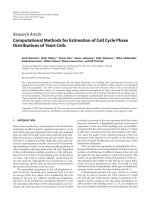
Basic to phase field theories are continuous field variables φ1 (x, t), φ2 (x, t), . . . , φQ (x, t)
(referred to as order parameters) which are functions of material points x and time
t. In the context of polycrystalline materials, the order parameters represent the
volume fraction of grains of a particular orientation. A schematics microstructure
represented by the orientation fields in 2-D is shown as in fig (3.1).

Figure 3.1: Representation of Orientation field variable φ

14