Constraint based method for finding motifs in DNA sequences
Bạn đang xem bản rút gọn của tài liệu. Xem và tải ngay bản đầy đủ của tài liệu tại đây (484.77 KB, 80 trang )
CONSTRAINT BASED METHOD FOR FINDING MOTIFS
IN DNA SEQUENCES
DONG XIAOAN
(Bachelor of Management, Wuhan University, China)
A THESIS SUBMITTED FOR
THE DEGREE OF MASTER OF SCIENCE
DEPARTMENT OF COMPUTER SCIENCE
NATIONAL UNIVERSITY OF SINGAPORE
2004
Acknowledgements
I would like to express my gratitude to all those who gave me the possibility to complete this thesis. My primary thanks go to my supervisor, Prof.
Sung Sam Yuan, for his invaluable guidance and advice throughout my
research. His priceless support has helped me all the time in the research.
I deeply appreciate Dr. Sung Wing Kin for his constructive guidance
in my research. He shared with me his knowledge and tips in writing
research paper, and provided me friendly encouragement all the way.
I sincerely appreciate my good friends Fa Yuan, Tang Jiajun, Yang Xia,
Chen Yabing, Zhou Yongluan, Li Jianer, Zhang Xi. They have helped
me in one way or other and made my study and research experience
unforgettable.
Last but not least, I am grateful to my parents for their patience and
love. Without them this work would never have come into existence.
i
Contents
Summary
iv
1 Background
1
1.1
Road Map to the thesis . . . . . . . . . . . . . . . . . . . .
3
1.2
Biological Background: DNA and Sequence Features . . .
4
1.2.1
DNA and Genomic Sequence . . . . . . . . . . . . .
5
1.2.2
Regulatory Sites - a Feature of Genomic Sequence .
7
1.3
Finding Sequence Features based on Sequence Similarity . 11
2 A Survey of Motif Finding Algorithms
15
2.1
Problem Definition . . . . . . . . . . . . . . . . . . . . . . 15
2.2
Motif Models: Strengths and Limitations . . . . . . . . . . 17
2.2.1
Consensus Model . . . . . . . . . . . . . . . . . . . 18
2.2.2
Weight Matrix Model . . . . . . . . . . . . . . . . . 19
2.2.3
Multi-positional Profile Model . . . . . . . . . . . . 21
2.2.4
Constraint based Model . . . . . . . . . . . . . . . 23
2.3
Motif Finding Algorithms . . . . . . . . . . . . . . . . . . 25
2.4
Significance of the Thesis Revisited . . . . . . . . . . . . . 27
3 Finding Motif using Constrain Based Method
3.1
29
Preliminaries . . . . . . . . . . . . . . . . . . . . . . . . . 30
ii
CONTENTS
3.2
3.3
Constraint Mechanism . . . . . . . . . . . . . . . . . . . . 31
3.2.1
The Basic Algorithm . . . . . . . . . . . . . . . . . 32
3.2.2
Heuristic Improvement . . . . . . . . . . . . . . . . 34
CMMF - Constraint Mechanism-based Motif Finding Algorithm . . . . . . . . . . . . . . . . . . . . . . . . . . . . 37
3.4
Constraint Rules . . . . . . . . . . . . . . . . . . . . . . . 39
3.5
CRMF - Constraint Rules-based Motif Finding Algorithm
3.6
Implementation Issues . . . . . . . . . . . . . . . . . . . . 46
44
3.6.1
Hamming Distance Matrix . . . . . . . . . . . . . . 47
3.6.2
Clique Conversion Threshold . . . . . . . . . . . . . 48
3.6.3
Duplicated Centers Elimination . . . . . . . . . . . 48
3.6.4
Center Testing . . . . . . . . . . . . . . . . . . . . 49
4 Experimental Results
52
4.1
Performance of CMMF and CRMF on Synthetic Data . . . 53
4.2
Challengeing Problems on Simulated Data . . . . . . . . . 55
4.3
Benchmarking . . . . . . . . . . . . . . . . . . . . . . . . . 57
4.4
Finding Motifs in Realistic Biological Data
. . . . . . . . 58
5 Conclusions and Open Problems
61
References
63
A Glossary
69
iii
Summary
Pattern discovery in unaligned DNA sequences is a fundamental problem
in both computer science and molecular biology. It has important applications in locating regulatory sites and drug target identification. This
thesis introduces two novel motif discovery algorithms based on the use of
constraint mechanism and constraint rules respectively. The key idea is
to convert sets of similar substrings on the DNA sequences into patterns,
as early as possible, using constraint mechanism or constraint rules. The
advantages are two folds. Firstly, the approach generates limited number
of patterns while still guaranteeing that the actual motifs are contained
in the pattern set. Secondly, the procedure for deriving patterns is very
cost-effective since it can be considered as that we use many “look ahead”
to speed up the procedure. Therefore, the algorithms have the advantages
of the high sensitivity of pattern-driven algorithms as well as the efficiency
of sample-driven algorithms.
iv
Chapter 1
Background
The history behind motif discovery in unaligned DNA sequences dates
back to 1970, when Hamilton Smith [18] discovered the Hind
restriction
enzyme. It may have been the first DNA pattern. This discovery provided
biological scientists with a new technological tool to study DNA sequences
in a more efficient manner.
Since the dawn of the 21st century, there has been a dramatic increase
in the number of completely sequenced genomes due to the efforts of both
public genome agencies and the pharmaceutical industries. Large-scale
genomics have become a fundamental tool for understanding an organism’s biology. Access to multiple complete genomic sequences helps biologists to formulate and test hypotheses about how genomes are organized
and evolved, as well as how a genome encodes the observed properties
of a living organism. Key questions being pursued include: what parts
of our genome encode the mechanisms for major cellular functions like
metabolism, differentiation, proliferation, and programmed death? How
do multiple genes act together to perform specialized functions? How is
our non-protein-coding DNA organized, and which parts of it are func-
1
CHAPTER 1. BACKGROUND
tionally important? How do selective pressures act on the random processes of gene duplication and mutation to give rise to complex constructs
like eyes, wings, and brains? Why do humans appear so different from
worms and flies, despite sharing so many of the same genes?
Until the 1990’s, molecular biologists could pursue questions about the
content and function of genomes only indirectly, or else at great cost. Indirect techniques such as Giemsa staining and CoT-based measurement of
repetitive content [45] provided limited information about a genome. Full
sequence was available for only a few short regions found to be functionally significant, usually after a long and expensive process of localization
by (e.g.) linkage mapping, followed by cloning out and finally sequencing
a minimal region of interest. The cost and time required to sequence
DNA made sequencing a tool to be applied only at particular points, and
only once a region was shown to be important by other means.
More recently, high-throughput DNA sequencing has enabled a direct
approach to studying genomes. Using this new technology, biologists have
obtained progressively larger complete genomic sequences, from viruses
[11] to prokaryotes [36] to single-celled [19] and multicellular [1] eukaryotes. Available genomes today include those of several higher metazoans,
including the fruit fly Drosophila melanogaster [31], the flowering plant
Arabidopsis thaliana [2], and, of course, Homo sapiens [3]. Armed with
substantially complete euchromatic sequences from these organisms, we
can now directly interrogate global properties like base frequencies and
repetitive content, obtain immediately the sequence of any potentially
interesting region, and perhaps most exciting compare corresponding
long stretches of genomic DNA in two or more organisms. Such analysis
encompass massive amounts of sequence, on a scale requiring computa2
CHAPTER 1. BACKGROUND
tion that defies manual analysis. The need to automate analysis of long
or numerous genomic sequences gives rise to the field of computational
genomics.
In this work, we address a particular problem of computational genomics: how to discover which parts of a long DNA sequence encode
particular biological features, such as genes. Even when the whole sequence is available for inspection, finding these features reliably can be
surprisingly difficult. If we know little about the features being sought,
or their presence leaves only a weak imprint on the underlying sequence,
finding them may be theoretically intractable or practically beyond our
limited budget of computing time and space. This work focuses specifically on new techniques to find features that are difficult to find in theory
or simply intractable to existing search algorithms.
The algorithms that we introduce in this thesis are founded on two
novel techniques, constraint mechanism and constraint rules, which extract patterns from sets of similar strings. We show how to exploit the
power of them to find motifs efficiently. As a result, we can more readily
identify more interesting features and ultimately provide more knowledge
to biologists.
1.1
Road Map to the thesis
We begin by providing the reader with a brief guide to the content of the
thesis. Some readers may find the biological terms used in subsequent
sections and chapters unfamiliar; hereafter, we will both define such terms
at their point of first use and provide a glossary (see Appendix A) of terms
to collect the important definitions in one place.
3
CHAPTER 1. BACKGROUND
Chapter 1 is devoted to background and significance. We first review the nature of genomic DNA. Then we introduce interesting features
which our algorithms focus on. Finally we introduce the basic approach,
sequence similarity comparison, to identify sequence features.
Chapter 2 is devoted to review the existing research work on motif
finding. We first present the formal definition of planted motif finding
problem, then we analyze the critical techniques - motif models - used for
pattern extraction. Based on the analysis, we review the existing motif
finding algorithms. Finally we revisit the significance of our algorithms.
Chapter 3 introduces two novel algorithms, namely constraint mechanismbased motif finding algorithm (CMMF) and constraint rules-based motif
finding algorithm (CRMF). We then show how to implement the algorithms in practice.
Chapter 4 presents the experimental results on both synthetic data
and biological data. Based on the results, we compare CMMF with
CRMF, and we also compare our algorithms with other leading motif
finding algorithms.
Chapter 5 summarizes the merits as well as limitations of our work.
We propose the ways to extend the algorithms to achieve better performance and pose the open problems as well.
1.2
Biological Background: DNA and Sequence Features
The first prerequisite to developing algorithms for finding features in genomic sequences is to understand what we are looking for and why. We
4
CHAPTER 1. BACKGROUND
therefore begin with a brief review of genomic DNA and its major features.
Readers seeking more background on genomic DNA or on molecular biology in general may wish to consult the standard text by Lewin [29] or
the gentler introduction by Joao Setubal and Joao Meidanis [40].
1.2.1
DNA and Genomic Sequence
The information encoded in genetic material, DeoxyriboNucleic Acid (DNA),
is responsible for establishing and maintaining the cellular and biochemical functions of an organism. In most organisms, the DNA (see Figure
1.1) is an extended double-stranded polymer composed of a sequence of
nucleotides, also called bases. Four such bases - A(Adenine), C(Cytosine),
G(Guanine), and T(Thymine) - form the alphabet from which all natural
DNA is constructed. Abstractly, a DNA sequence is simply a string over
the alphabet {A,C,G,T}. We will use the terms “string” and “sequence”
interchangeably.
The sequence of bases of one DNA strand is complementary to the
bases of the other strand. This complementarity enables new DNA molecules
to be synthesized with the same linear array of bases in each strand as
an original DNA molecule. The process of DNA synthesis is called replication, which plays a critical role in passing on genetic information from
one generation to the next. Complementary bases forms base pairs. The
pairing is deterministic: A always pairs with T, while C pairs with G.
Thus, the sequence of one strand determines the sequence of its complement, and we can describe a DNA sequence uniquely by only one of
its strands. Because of this pairing, bases are sometimes classified as
“weak” (A/T, joined by two hydrogen bonds) or “strong” (C/G, joined
by three hydrogen bonds). Another common classification of bases, this
5
CHAPTER 1. BACKGROUND
Figure 1.1: Double Stranded DNA Model
time by chemical structure, is as purine (A/G) or pyrimidine (C/T). An
unspecified purine or pyrimidine is denoted by the characters R and Y
respectively.
DNA either swims within the cytoplasm of prokaryotic cells (e.g. bacteria and E.coli) or locates within the nucleus of eukaryotic cells (e.g.
plant and animal). An organism’s complete set of DNA sequence is its
genome. The differences in genomic sequence from one organism to another within a species are quite small compared to the differences between
species, so it makes sense to talk about an entire species’ genome. For example, the human genome, which is 3 × 10⁹ base pairs in length, is 99.9%
similar between individuals, while the genome of our closest relative, the
chimpanzee, is only 98% - 99% similar to ours [8].
An organism’s genome is organized into a small number of discrete
DNA molecules, called chromosomes. Bacteria typically have a single,
6
CHAPTER 1. BACKGROUND
circular chromosome a few million bases in length, while eukaryotic species
have anywhere from three to over 100 linear chromosomes of total length
ranging from tens of millions up to billions of bases.
An essential feature of DNA is that it is not static over time. Chemicals, radiation, and copying errors can all cause a DNA sequence to
mutate. Biologically common types of mutation include substitutions, in
which one base is replaced by another, and indels (insertions and deletions), in which bases are added to or removed from a sequence. Different
types of mutation happen at different rates; for example, transition substitutions - those that replace A with G or C with T and vice versa are roughly twice as common [9] as other substitutions, which are called
transversion.
1.2.2
Regulatory Sites - a Feature of Genomic Sequence
Most sequence features fall broadly into three categories: genes, which
encode the active molecules that carry out the cell’s business; regulatory
sites, which control the behavior of genes; and repetitive elements. Our
algorithms focus on finding regulatory sites, which will be introduced in
detail at follows.
Regulatory sites control the behavior of genes. Precisely, regulatory
sites control when and where genes are expressed to produce their products. It is necessary to know genes before we illustrate regulatory sites.
Genes are the basic physical and functional units of heredity. A gene
is a specific sequence of bases, which encode instructions for building other
polymeric molecular species. A gene’s basic function is to have its DNA
7
CHAPTER 1. BACKGROUND
sequence transcribed into a corresponding (single-stranded) polymer of
RNA, or RiboNucleic Acid. The sequence of an RNA molecule is identical
to that of its originating gene, except that T bases are mapped not to T
but rather to a different base, U (Uracil).
Cells have regulatory mechanisms for controlling when and where
genes are expressed to produce their products. Sets of short stretches
of base pairs (signal regions) within the DNA are required to ensure that
gene expression is initiated at the correct nucleotide and that it terminates at a specific nucleotide. The sequences that control the initiation
of gene expression usually precede the coding sequence, and termination
signal sequences follow it. Figure 1.2 illustrate how a structural gene in
prokaryotes is transcribed into mRNA [16], which then is translated into
protein. In prokaryotes, a contiguous DNA segment forms a structural
gene. Prokaryotic transcription entails the binding of RNA polymerase
to a promoter region, the initiation of transcription at the first nucleotide
of the gene, and the cessation of transcription at a termination sequence
that lies downstream from the coding region.
In this work, we focus on one particular form of regulation: control
of gene transcription by a class of proteins called transcription factors.
These proteins adhere to genomic DNA at binding sites, regions up to a
few tens of bases in length that contain factor-specific signal sequences.
Transcription factors often bind at sites within a few hundred bases at
the start of a gene, where they influence how frequently the RNA polymerase complex initiates transcription of that gene. These sites are called
enhancer/repressor regions. If a transcription factor causes the gene to be
expressed at a higher level, it is said to be an enhancer; if it causes a lower
level of expression, it is a repressor. Figure 1.3 illustrates how a repressor
8
CHAPTER 1. BACKGROUND
upstream region
dow nstream region
Figure 1.2: Prokaryotic Transcription. Schematic representation of a
prokaryotic structural gene. The promoter region (p), the site of initiation and direction of transcription (the right-angled arrow), and the termination sequence for RNA polymerase (t) are depicted. A prokaryotic
structural gene is transcribed into mRNA and then directly into protein.
protein binds to a regular binding site to block the transcription.
Transcription factors are often activated in response to changes in the
cell’s environment, especially changes in the amounts of various chemicals (including other gene products). These proteins can therefore orchestrate the cell’s transcriptional response to changing external conditions as
well as carrying out “programs” such as cell division, differentiation, or
death in response to particular chemical signals. The exact mechanism by
which transcription factors transduce these changes varies. Many factors
form (or block formation of) protein complexes that contact the RNA
polymerase directly, increasing or decreasing its affinity for binding to a
gene’s promoter and initiating transcription [29]. Factors may also alter
the conformation of the DNA to which they bind, again changing the
binding affinity of the polymerase [38, 39].
9
CHAPTER 1. BACKGROUND
Prom oter Region
RN A
p o ly m erase
A:
Binding
Site
R
No Transcription
Gene
T erm ination
Signal Sequenc e
t
DNA
R
: Repressor Protein
Transcription
RN A
p o ly m erase
B:
Gene
t
DNA
Figure 1.3: Schematic representation of a bacterial transcription unit.
Transcription is catalyzed by RNA polymerase. In Figure A, the repressor
protein (R) binds to the regular binding site and blocks transcription. In
Figure B, the repressor protein can not bind to the binding site due to
some chemical changes, thus RNA polymerase can transcribe the gene.
Multiple transcription factors can act on a single gene, in which case
several different binding sites may cluster near that gene. The factors’
actions are not necessarily independent; in general, they may form a
complex cis-regulatory logic that permits fine control over when and how
strongly a gene is expressed. At this time, few examples of cis-regulatory
logic have been worked out in detail; the work of Yuh et al. in sea urchin
development [53] illustrates the complexity possible in such logic.
Transcription factor binding sites, while clearly are important sequence features. Unfortunately, they are difficult to identify in raw genomic sequence. We know that sites are likely to occur in clusters in the
promoter regions of genes, typically within a few hundred to a few thousand bases of the transcription start site. However, significant sites may
be found elsewhere, including the introns of genes [23] and locus control
regions that may be ten kilobases (ten thousand bases) or more away
10
CHAPTER 1. BACKGROUND
from the genes they regulate [14]. In general, we cannot assume much
a priori about what binding sites look like - their sequence patterns are
too dependent on the particular factor that they bind. Certain types of
transcription factor may require binding sites with known structure, such
as a DNA palindrome for some homodimeric factors, but such structures
are far from universal.
Finally, we note that even if all the sites for a given transcription factor had identical sequence (which is not the case), the sequence pattern
is usually short enough that it may occur purely by chance in the background sequence, at a place where no protein actually binds. Programs
to find new transcription factor binding sites in genomic sequences are
therefore challenged not only by a lack of identifying characteristics for
these sites but also by confusions between true binding sites and chance
occurrences of their sequence patterns.
1.3
Finding Sequence Features based on Sequence Similarity
We now come to the vital problem of identifying features in raw DNA
sequence. There is well-known conjecture that in the industry of biology
that, if two DNA sequence are highly similar, we can infer that they share
similar function. Consequently, researchers of bioinformatics can find
interesting sequence features through comparing the similarity between
two or more biological sequences.
The similarity between the occurrences of a feature is due to its conservation, or lack of change, over evolutionary time. Although all DNA
11
CHAPTER 1. BACKGROUND
sequences are subject to mutation, natural selection ensures that we observe today only those individuals whose ancestors’ reproductive fitness
was not limited by strongly deleterious mutations. Many mutations to
genes or regulatory elements can render them dysfunctional, causing the
organism carrying these mutations to die or to have fewer viable offspring. In contrast, mutations in nonfunctional sequence can accumulate
freely with no effect on reproductive fitness. We therefore expect that
the organisms we see today exhibit fewer mutations, or equivalently more
conservation, in their functional sequences than in their background sequence.
Sequence alignment is a quantitative measure of similarity. Suppose
that some ancestral DNA sequence s0 evolves by mutation along two
separate lineages, creating present-day sequences s1 and s2 . If we knew
the entire mutation history of s1 and s2 , we could match up those bases
in each sequence that derive from the same ancestral base of s0 . Figure
1.4 shows such a matching, or alignment, of two sequences, written as a
series of columns in which bases deriving from the same ancestor appear
in the same column. If, as in this example, the sequences are subject to
indels, the alignment contains gaps, represented in the figure by columns
containing dashes “−”, where bases in one sequence do not correspond
to any part of the other sequence.
The goodness of alignment is defined by
i
δ(s1 [i], s2 [i]), where δ(x, y)
is a similarity function between x and y, each is a single base or a single
space. e.g., δ(x, y) = 2, −1, −1, −1 for match, dismatch, delete and insert respectively. In the example illustrated in Figure 1.4, We can check
that the optimal alignment has the maximal score. An optimal alignment between two sequences can be computed using global alignment, in
12
CHAPTER 1. BACKGROUND
T rue
Mutatio n
Histo ry
O p timal
Alignment
S0 :
..
..
AC GGG T T C C AG T AC
.
.
S1 :
..
..
A * GGG T aCC AGC T AC
.
.
S2 :
..
..
ACGG c T T CC t C G T AC
.
.
S1 :
..
..
A - GGG T A C C AG C - T A C
.
.
S2 :
..
..
ACGGC T T C C T - CG T AC
.
.
Figure 1.4: Example of a optimal alignment between two DNA sequences
s1 and s2 with a common ancestor s0 . In the true mutation history, lowercase letters indicate substitutions, while underlined bases and “∗” indicate
insertions and deletions. In the optimal alignment, some spaces, indicated
by “−”, are introduced to match as much as letters in the two sequences.
Note that the best alignment of the sequences is historically incorrect. The
two bases, indicated by arrow, do not derive from the same ancestral base.
particular the Needleman- Wunsch dynamic programming algorithm [33].
Features are always embedded in long genomic sequences. Compared
with features, background sequences are either wholly unrelated or so illconserved as to be unalignable. To find short and well-conserved features
in long background sequences, we can use local alignment, in particular
the Smith-Waterman dynamic programming algorithm [47], which ignore
the background sequence and measuring only the similarity between features.
As shown in the Figure 1.4, even the optimal alignment may not reflect
the true history of two sequences. The fact is that, the history of modern
genomic sequence is unknown, and what we can do is to plausibly guess
at the true matching of bases by finding an optimal alignment.
13
CHAPTER 1. BACKGROUND
Sequence similarity forms the basis to find interesting features in long
genomic sequences. Similar substrings between sequences are considered
as possible occurrences of a feature. Based on such substrings, we derive the possible feature and verify it globally against all background
sequences.
14
Chapter 2
A Survey of Motif Finding
Algorithms
In this chapter, we first formalize the motif finding problem. Then we
analyze the critical techniques - motif models - used for pattern extraction,
and discuss their strengths and limitations respectively. Based on the
analysis, we review the existing motif finding algorithms. Finally we
revisit the significance of our algorithms. Note that we focus specifically
on the widely studied problem of finding regulatory motifs in genomic
sequence by ungapped multiple local alignment.
2.1
Problem Definition
A motif is a conserved DNA sequence pattern recognized by a transcription factor or by other cellular machinery. The conservation of a regulatory motif across organisms or across genes allows us to identify it through
similarity search. However, since regulatory motifs are so short and are
imperfectly conserved, limited occurrences of a motif by themselves may
15
CHAPTER 2. A SURVEY OF MOTIF FINDING ALGORITHMS
not provide significant evidence of conservation. For example, consider
the problem of finding two occurrences of a conserved 20-mer motif that
differ by only five substitutions, in a pair of 1-kb background sequences
that are randomly generated with equal base frequencies. The expected
number of 20-mer matches with at most five substitutions appearing by
chance in the background is about 3.67, so two occurrences of the motif
would be indistinguishable from the background. Unless we can localize
the motif to a very much smaller region, the only way to demonstrate its
significance is to find additional occurrences in other sequences.
Following Buhler & Tompa [7], the formal definition of the motif discovery problem can be as follows.
Planted (l, d) - Motif Problem: Consider a set E of t nucleotide sequences each of length n. Suppose there is a fixed but unknown nucleotide
sequence M (motif) of length l which is implanted in every sequence of E.
The motif discovery problem is to determine M given E. More precisely,
the problem is to compute M such that every sequence in E contains a
length-l substring which has at most d mismatches when compared with
M.
Note that there are two widely used consensus based motif models,
where the motif consists of instances which are mutated occurrences of
the motif skeleton. One is FM model [35] where each of the t sequences
contains one instance of an (l,d)-motif. The other one is VM model [35]
where again each sequence contains exactly one instance, only now each
position of the instance is mutated, independently of all other positions,
with probability ρ. Due to our work concentrate on the first model, it is
used in the above formulation of motif problem.
16
CHAPTER 2. A SURVEY OF MOTIF FINDING ALGORITHMS
2.2
Motif Models: Strengths and Limitations
It is always difficult to identify all the occurrences of a conserved motif
without any information of the motif, especially in the case of substantive background sequences. Most existing algorithms capture the motif
skeleton, an estimated motif, through collecting partial occurrences as a
start, then we try to find additional occurrences against the whole background to restore the motif. Obviously the procedure of extracting out
the motif skeleton from partial occurrences plays an critical role in deciding the accuracy of these algorithms. And this procedure is more often
called as pattern extraction. Many different pattern extraction methods
exist for multiple sequences [17]. However what we focus on are not these
methods themselves, but several underlying motif models commonly used
in these methods. They are consensus model, the profile or weight matrix model (WMM) and multiprofile model. We also introduce constraint
based model used in our algorithms.
It is assumed that the occurrences of a motif may differ only by substitutions, not by indels (insertions or deletions) in the above four models.
This assumption reflects (1) the limitations of many computational technologies for finding motifs and (2) the fact that biologically interesting
motifs are frequently ungapped. Some known motifs consist of a small
number of ungapped segments with intervening variable-length spacers
[26, 41]; such motifs can be modelled as a collection of ungapped consensus whose occurrences always appear near each other with gaps of varying
length.
17
CHAPTER 2. A SURVEY OF MOTIF FINDING ALGORITHMS
2.2.1
Consensus Model
The consensus model is a simple combinatorial description of a motif.
In this model, the motif is considered as a consensus sequence. Each
occurrence of the motif is a copy of the consensus sequence, perhaps with
a few substitutions. Given multiple occurrences of a motif, the consensus
sequence can be formed as follows. The consensus at each position of
multiple sequences is defined as the base which occurs most often at
the position. In the case that two or more bases have equal highest
occurrences at a position, the consensus can be chosen randomly from
these bases. And the consensus sequence consists of the consensuses at
each position as illustrated in Figure 2.1.
5 occurrences of a motif
Consensus Sequence
C A T C A A T
T G C T A A T
TGTCAAT
T G T A C A T
T G G C A C T
T G T T G A T
Figure 2.1: A consensus model inferred from five occurrences of a motif.
The most frequent base in each position of the occurrences becomes the
base of the consensus at the position. If two or more bases appear equally
often in a given position, as with T and C in the fourth position, the
choice of the consensus base at that position is arbitrary.
One could measure the conservation of a motif by the number of substitutions between each occurrence and the consensus sequence.
Strength. Consensus model is the simplest model. Given multiple occurrences, it extract a single pattern - consensus sequence. In most cases, it
is effective in the sense that the base that appears most frequently in each
18
CHAPTER 2. A SURVEY OF MOTIF FINDING ALGORITHMS
position has the highest likelihood to be the original base of the motif.
Limitation. Consensus model risks missing the actual motif. This happens in the situation that the base at any position of the motif is badly
conserved in its occurrences.
2.2.2
Weight Matrix Model
The consensus model is uninformative due to that it does not reveal
either how strongly the consensus base in each position is conserved or the
distribution of non-consensus bases. However, all these information are
described in the weight matrix model (WMM), also called profile model.
WMM is a probabilistic model, which models a motif of length l as a 4 × l
matrix M , where the entry at position M [p, q] gives the probability that
an occurrence of the motif contains a base q (q = A,C,G,T ) in its pth
position. Each column of the matrix therefore sums to one as illustrated in
Figure 2.2. The distribution of bases in different positions are independent
of each other. Given a length-l sequence s, let s[i] denotes the base at its
ith position. Based on the weight matrix, the probability that M produces
a particular length-l motif instance m is : P r[ m | W ] =
l
W [ m[i], i ].
i=1
Given a set of motif occurrences M , the weight matrix W [ M ] can be
easily computed by calculating the frequency of each base in each position.
The weight matrix of the five motif occurrences in Figure 2.1 is shown in
Figure 2.2.
The matrix W [ M ] is the best description of M in the sense of
maximum likelihood. It is the WMM W that maximizes the likelihood
L[ W [M ] | M ] =
P r[ m | W ]. And the likelihood L[ W [M ] | M ] is
m∈M
also a useful score by which to measure the extent of conservation of the
19
CHAPTER 2. A SURVEY OF MOTIF FINDING ALGORITHMS
5 occurrences of a motif
Weight Matrix
1
C A T C A A T
T G C T A A T
T G T A C A T
T G G C A C T
T G T T G A T
2
3
4
5
6
7
A
C 0.2 0 0.2 0.4 0.2 0.2 0
G 0 0.8 0.2 0 0.2 0 0
T 0.8 0 0.6 0.4 0 0 1
0 0.2 0 0.2 0.6 0.8 0
Figure 2.2: A weight matrix model (WMM). It is inferred from the five
motif occurrences in Figure 2.1. Entries corresponding to the consensus
base at each position are identified in bold face. Unlike the consensus
model, the WMM captures the frequencies of both consensus base and nonconsensus bases, and it remains well-defined even when the consensus base
is ambiguous, as in the fourth position.
motif.
If the motif occurs in random background sequences with a base distribution P , a better scoring function for the set M of motif occurrences
is the likelihood ratio LR(M ), defined as
LR(M ) =
L[ W (M ) | M ]
L[ P | M ]
where
L[ P | M ] =
P r[ m | P ]
m∈M
The likelihood ratio, while is not strictly a measure of conservation, is
a principled way to account for the background base distribution when
scoring a motif. The ratio adjusts for the background distribution by
recognizing that, if base i appears frequently in the background, then a
collection of strings with a high frequency of i’s is more likely to occur
purely by chance, and is therefore less significant as a putative motif, than
one with few i’s.
Strength. WMM is a probabilistic model, which captures the frequencies
20