Effect of suspended sediment on turbulent velocity profiles in open channel flows
Bạn đang xem bản rút gọn của tài liệu. Xem và tải ngay bản đầy đủ của tài liệu tại đây (1.23 MB, 138 trang )
EFFECT OF SUSPENDED SEDIMENT ON TURBULENT VELOCITY
PROFILES IN OPEN-CHANNEL FLOWS
TIN MIN THANT
NATIONAL UNIVERSITY OF SINGAPORE
2003
EFFECT OF SUSPENDED SEDIMENT ON TURBULENT
VELOCITY PROFILES IN OPEN-CHANNEL FLOWS
TIN MIN THANT
(B.Eng.(Civil),YTU)
A THESIS SUBMITTED
FOR THE DEGREE OF MASTER OF ENGINEERING
DEPARTMENT OF CIVIL ENGINEERING
NATIONAL UNIVERSITY OF SINGAPORE
2003
ACKNOWLEDGMENTS
The author would like to express his appreciation a number of people who have
contributed, directly or indirectly, to this thesis. First and foremost, the author would like to
express gratitude and appreciation to Assistant Professor Guo Junke, John, his supervisor, for his
guidance, encouragement, friendship and support during this study as well as for sharing his wide
knowledge of fluid mechanics.
His never failing optimism and his steadfast support and
assistance were the keys toward the successful completion of this thesis.
The experimental data used in this thesis are provided by some researchers. These people
are greatly acknowledged. Their valuable data sets are certainly important for this study.
The author gratefully the help and friendship received from his colleagues and friends
during the course of the study.
The author is also very much indebted to the National University of Singapore for
providing a Research Scholarship that made his studies possible at the Department of Civil
Engineering.
Finally, the author would like to dedicate this work to his parents who brought him to his
level and hence his special thank are due to them. The author would also like to dedicate this
thesis to his wife May Kyee Myint and his son Lu Lu for their patience, understanding, and love
through the two years required for this effort.
ii
TABLE OF CONTENTS
ACKNOWLEDGEMENT
ii
TABLE OF CONTENTS
iii
SUMMARY
vii
NOMENCLATURE
ix
LIST OF FIGURES
xiii
LIST OF TABLES
xv
CHAPTER 1
INTRODUCTION
1.1
General statement of the subject
1
1.2
Background of study
2
1.3
Objectives
3
1.4
Outline of the present study
4
CHAPTER 2
LITERATURE REVIEW
2.1
Introduction
5
2.2
Velocity profiles for clear water
5
2.2.1 Linear Law
6
2.2.2 Log Law
9
2.2.3 Power Law
11
2.2.4 Log wake Law
13
2.2.5 Modified Log-wake law
17
2.3
Velocity profiles of Sediment-laden flow
2.3.1 Log law in sediment-laden flows
iii
19
2.3.2 Power law in sediment-laden flows
21
2.3.3 Log wake law in sediment-laden flows
22
2.3.4 Modified log-wake law in sediment-laden flow
24
2.4
Log linear law and others
24
2.5
Concentration profiles
27
CHAPTER 3
MODELLING THE LOGARITHMIC MATCHING
EQUATIONS
3.1
Introduction
30
3.2
Logarithmic matching method
30
3.3
Analysis by asymptotic method to logarithmic matching equations
33
3.3.1 Analysis by log laws
33
3.3.2 Analysis by power laws
37
CHAPTER 4
TEST OF THE LOGARTHMIC MATCHING EQUACTION
IN SEDIMENT-LADEN FLOW
4.1
Introduction
41
4.2
Test of the logarithmic matching equation (1) in open-channel
41
4.2.1 Data selection
41
4.2.2 Methods for determining parameters
43
4.2.3 Test the structure of log matching equation (1)
44
Test the effect of sediment suspension on model parameters
49
4.3.1 The von Karman constant,κm
49
4.3.2 Integration constant C1
50
4.3.3 The matching parameter, x0
52
4.3
iv
4.4
4.5
Test of the logarithmic matching equation (2) in open-channel
53
4.4.1 Data selection
53
4.4.2 Method for determining parameters
54
4.4.3 Test the structure of log matching equation (2)
55
Test the effect of sediment suspension on the model parameters
61
4.5.1 The exponential constant, γ1
62
4.5.2 The power law constant α1
63
CHAPTER 5
SUSPENDED SEDIMENT IN OPEN-CHANNEL FLOWS
5.1
Introduction
65
5.2
Equation for relative concentration distribution
66
5.3
Test the relative equations on Coleman's (1986) data
68
5.4
Test the parameter with w/u* and Richardson number, Ri
71
5.4.1 The exponential parameter γ
74
5.4.2 The parameter α
75
5.4.3 The parameter B
75
CHAPTER 6
CONCLUSIONS
6.1
Summary
77
6.2
Conclusions
78
81
REFERENCES
APPENDIX A: MATLAB PROGRAMS
Program for solving parameters in the logarithmic matching equation
v
90
APPENDIX B: ANALYSIS OF EINSTEIN AND CHIEN 'S (1955)
EXPERIMENTAL DATA
Introduction
99
Velocity profile analysis
100
APPENDIX C: ANALYSIS OF COLEMAN'S (1986) VELOCITY PROFILES
Introduction
106
Velocity profile analysis
107
APPENDIX D: ANALYSIS OF COLEMAN'S (1986) CONCENTRATION
PROFILES
Introduction
113
Concentration profile analysis
114
vi
SUMMARY
EFFECT OF SUSPENDED SEDIMENT ON TURBULENT VELOCITY
PROFILES IN OPEN-CHANNEL FLOWS
This thesis studies turbulent velocity profiles in open-channel for sediment-laden flows.
The main purpose is to test a suitable velocity profile function for the whole turbulent
flow layer by using logarithmic matching method and to study the effects of sediment
suspension on the model parameters.
Basically, the logarithmic matching method
combines two asymptotes, in extreme case, which can be expressed as the logarithmic or
power laws, into a single composite solution. The composite equation has three terms, a
log term, a linear term and a function which could be consider as a wake function in
sediment laden flow.
The major findings are:
We introduce two suitable velocity profile models for the whole turbulent flow
layer by using logarithmic matching method and to study the effects of sediment
suspension on the model parameters. Model (1) is analyzed by two logarithmic laws and
Model (2) is analyzed by two power laws.
A model (1) turbulent velocity profile
equation, a composite equation, consists of three parts: a log term, a linear term and a
linear function. Model (2) velocity profile equation consists of exponential or power
term.
These two velocity profile equations are referred to as the logarithmic matching
equations (1) and (2). The new equations consider the whole layer.
vii
The logarithmic matching equations agree well with experimental data for
sediment-laden flow in the whole flow layer. Sediment suspension affected on the
velocity profile in two factors: sediment concentration and density gradient (the
Richardson number Ri).
The flow with sediment can be divided into an inner suspension region near the
bed and an outer region in the free stream, with the properties of the sediment transfer
process being different in the two zones. The relating concentration profile models are
established for these two regions based on the logarithmic law and the power law.
In our work, we use the Gauss-Newton nonlinear optimization method to find the
parameters. The logarithmic matching equation (1) contains four parameters: (1) the von
Karman constant in near bed region κ = 0.4; (2) the von Karman constant in main flow
region κm which is less than 0.4; (3) the integration constant C1; and (4) the matching
parameter x0.
The logarithmic matching equation (2) contains two parameters: the exponential
parameter γ1 and the power law constant α1.
The concentration profile equation which is related for inner region is established
by power law. It has two parameters: the exponential parameter γ and the power law
constant α. The concentration profile equation of outer suspension region is modeled by
velocity defect law. It also has only one parameter B.
viii
NOMENCLATURE
A
integration constant
a
a reference of flow depth
B
another integration constant
C1, C2
integration constants in logarithmic law
C
mass concentration (g/l)
C
average sediment concentration
Ca
a reference sediment concentration
Cd
drag coefficient
Cv
volumetric concentration
Cw
concentration by weight
Cf
skin-friction coefficient
d
particle diameter
d50
median particle diameter
g
acceleration due to gravity
h
avg. depth of open-channel flow
K1, K2
slope constant
lm
Prandtl's mixing length
Re
Reynolds' number
ms
mass of sediment
S
channel slope
Se
energy slope
ix
T
temperature (ºF)
T0
absolute temperature
U
avg. flow velocity
u
velocity at a distance y from the bed
u
average velocity
u max
maximum velocity
u*
shear velocity
u',v',w'
velocity fluctuation
v x' v z'
average of absolute values of vx' , vz' respectively
Vs
settling velocity of the sediment particle
Vwind
wind velocity over the water
R
pipe radius
Rb
hydraulic radius
Re
Reynold number
Ri
Richardson number
x
coordinate of the downstream direction
x0
a reference of x
w
coordinate of the lateral direction
y
vertical distance from bed
y0
matching parameter
z
coordinate of the upward direction that is perpendicular to x-y plane
α
equation parameter
x
α1, α2
power law constants
γ1, γ2
exponential parameters
β
transitional shape parameter
ε 1+
dimensionless eddy viscosity at the water surface
εm
coefficient of momentum exchange
εs
diffusion coefficient of sediment
δ
boundary layer thickness, which is the distance form the bed to the
position of maximum velocity
ρ0
mass density of water
ρ
density of water-sediment mixture
ρs
density of the sediment
ρm
density of the sediment-laden flow
ρair
air density
П
wake strength
Ω0
wake strength for clear water
η
dimensionless distance form wall
λ
free surface factor
λ0
water surface shear effect factor
µ
dynamic viscosity of fluid
µ0
absolute viscosity
ν
kinematic viscosity
τ
shear stress
xi
τ0
bed shear stress
ξ
vertical distance from bed normalized by flow depth
γ
specific weight of water
γs
specific weight of sediment
γm
specific weight of sediment-laden flow
κ
von Karman constant
κ0
von Karman constant in clear water
κm
von Karman constant in main flow region, less than 0.4
ω
settling velocity
xii
LIST OF FIGURES
Figure 2.1
Sketch of a representative velocity profile in open-channels
Figure 2.2
A comparison between log law and power law for Reynolds numbers
6
between 31×103 and 4.46.
13
Figure 2.3
Mean velocity distribution in open-channel flows
14
Figure 2.4
Velocity-defect law in open-channel flows
16
Figure 3.1
The scheme of the logarithmic matching
31
Figure 3.2
Average concentration effect on the transition parameter β
36
Figure 3.3
Density gradient effects on the parameter γ2
39
Figure 3.4
Density gradient effects on the transition parameter β
39
Figure 3.5
Density gradient effects on the parameter α2
40
Figure 4.1
A representative velocity profile of sediment-laden flows in open-channel,
[(a) semilog coordinates; (b) Cartesian coordinates;]
Figure 4.2
Compare of log matching equation (1) with Einstein and Chien's (1955)
data
Figure 4.3
45
46
A representative velocity profile of Vanoni's (1946) data in sedimentladen flow [(a) Cartesian coordinates; (b) semilog coordinates;]
48
Figure 4.4
Compare of log matching equation (1) with Vanoni's (1946) data
48
Figure 4.5
Sediment concentration effect on the von Karman constant in main flow
region
50
Figure 4.6
Sediment concentration effect on the integration constant
52
Figure 4.7
Sediment concentration effect on the matching parameter
53
xiii
Figure 4.8
A representative velocity profile of sediment-laden flows for Coleman's
(1986) experimental data [(a) Loglog coordinates; (b) Cartesian
coordinates;]
Figure 4.9
56
Comparison of logarithmic matching equation (2) with Coleman's (1986)
experimental data.
Figure 4.10
57
A representative velocity profile of sediment-laden flows for Einstein and
Chien's (1955) experiment data. [ (a) Cartesian coordinates; (b) semilog
coordinates;]
Figure 4.11
60
Comparison of logarithmic matching equation (2) with Einstein and
Chien's (1955) experimental data
60
Figure 4.12
Density gradient effects on the exponential parameter γ1
63
Figure 4.13
Density gradient effects on power law constant α1
64
Figure 5.1
A representative typical concentration profile
66
Figure 5.2
Relationships between ln A and ln B.
68
Figure 5.3
Test the structure of the relative concentration profile equations. (a) in a
semilog coordinate system. (b) in a loglog coordinate system.]
69
Figure 5.4
Plot of the relationship between γ and ω/u*.
72
Figure 5.5
Plot of the relationship between α and ω/u*
73
Figure 5.6
Plot of the relationship between B and ω/u*.
73
Figure 5.7
Plot of the relationship between γ and Ri, Richardson number.
74
Figure 5.8
Plot of the relationship between α and Ri, Richardson number.
75
Figure 5.9
Plot of the relationship between B and Ri, Richardson number.
76
xiv
Figure B.1
A velocity profile of sediment-laden flow. [(a) Cartesian coordinates;
(b) semilog coordinates;]
Figure B.2
100
A velocity profile of sediment-laden flow. [(a) Cartesian coordinates;
(b) semilog coordinates;]
Figure B.3
101
A velocity profile of sediment-laden flow. [(a) Cartesian coordinates;
(b) semilog coordinates;]
Figure B.4
102
A velocity profile of sediment-laden flow. [(a) Cartesian coordinates;
(b) semilog coordinates;]
Figure B.5
103
A velocity profile of sediment-laden flow. [(a) Cartesian coordinates;
(b) semilog coordinates;]
Figure B.6
104
A velocity profile of sediment-laden flow. [(a) Cartesian coordinates;
(b) semilog coordinates;]
Figure C.1
105
A velocity profile of sediment-laden flow. [(a) log-log coordinates;
(b) Cartesian coordinates;]
Figure C.2
107
A velocity profile of sediment-laden flow. [(a) log-log coordinates;
(b) Cartesian coordinates;]
Figure C.3
108
A velocity profile of sediment-laden flow. [(a) log-log coordinates;
(b) Cartesian coordinates;]
Figure C.4
109
A velocity profile of sediment-laden flow. [(a) log-log coordinates;
(b) Cartesian coordinates;]
Figure C.5
110
A velocity profile of sediment-laden flow. [(a) log-log coordinates;
(b) Cartesian coordinates;]
111
xv
Figure C.6
A velocity profile of sediment-laden flow. [(a) log-log coordinates;
(b) Cartesian coordinates;]
Figure D.1
112
A concentration profile of sediment-laden flow.[(a) semilog coordinates;
(b) log-log coordinates;]
Figure D.2
114
A concentration profile of sediment-laden flow.[(a) semilog coordinates;
(b) log-log coordinates;]
Figure D.3
115
A concentration profile of sediment-laden flow.[(a) semilog coordinates;
(b) log-log coordinates;]
Figure D.4
116
A concentration profile of sediment-laden flow.[(a) semilog coordinates;
(b) log-log coordinates;]
Figure D.5
117
A concentration profile of sediment-laden flow.[(a) semilog coordinates;
(b) log-log coordinates;]
Figure D.6
118
A concentration profile of sediment-laden flow.[(a) semilog coordinates;
(b) log-log coordinates;]
119
xvi
LIST OF TABLES
Table 4.1
Calculated results of Einstein and Chien's (1955) experimental data
46
Table 4.2
Calculated results of Vanoni's (1946) experimental data
49
Table 4.3
Calculated results of Coleman's (1986) experimental data
58
Table 4.4
Calculated results of Einstein and Chien's (1955) experimental data for log
Table 5.1
matching equation (2)
61
The calculated results of Coleman's (1986) concentration profile data.
70
xvii
CHAPTER 1
INTRODUCTION
1.1
General Statement of the subject
Turbulent sediment-laden flows are of direct importance not only to river and
environmental engineering but also to other related areas, such as coastal sediment
transport and transport of materials in pipelines. Turbulent velocity profile is a basis
subject in fluid mechanics. Knowledge of turbulent velocity profiles in open-channel
flow is important analysis of resistance to flow, contaminant transport, and sediment
studies.
The turbulence in open-channel flows is very important in fundamental
hydraulics and fluid mechanics as well as in applied hydraulic engineering such as river
and estuary engineering. Despite of decades of intensive research, the mechanics of
sediment transport remains far from a complete physical or analytical description. At
present, even for clear water turbulent flows reliable information on the main flow
parameter (such as velocity and shear stress distributions) is available only for twodimension flows. Therefore, sediment-laden flows can be studied only for the simplest
case. This study addresses the problem: what is the best functional form of the velocity
profile equation in open-channel with sediment-laden flow and how does sediment
suspension affect the velocity profile. Its accurate prediction is helpful for the analysis of
a river development and management, reservoir operation, flood protection and etc.
1
1.2
Background of study
Although many investigations on velocity profiles have been reported for at least one
century, this subject is still very challenging. The interactions of suspended particles
with the underlying turbulent flows and resulting effects have remained challenging
problems in fluid mechanics. The well-known universal law of velocity distribution in
the turbulent boundary layer was deduced by Prandtl (1932) using mixing-length
hypothesis and by von Karman (1930) using the similarity hypothesis. The studies in
clear water include Nikuradse (1932), Keulegan (1938), Laufer (1954), Clauser (1956),
Patel and Head (1969), Nezu and Nagagawa (1993), Parahtasarathy and Muste (1993),
Zagarola (1996), Guo (1998) and many others. The studies in sediment-laden flows
include Vanoni (1946), Einstein and Chien (1955), Vanoni and Nomicos (1960), Elata
and Ippen (1961), Montes and Ippen (1973), Itakura and Kishi(1980), Lau (1983),
Coleman (1981, 1986), Karim and Kennedy (1987), Lyn (1986, 1988, 1991, 1992), Wang
and Qian(1989 ,1992), Barenblatt (1993), Muste and Patel (1997), Guo and Julien (2001)
and many others. They examined the log law, the log-wake law, and power law and
modified log-wake law describing the variation of velocity with depth in sediment-laden
flows. They concluded that the von Karman decreases and turbulence intensity increases
with increasing sediment concentration. Coleman (1986) pointed out that the previous
conclusion, i.e., κ decreases with sediment suspension, was obtained by incorrectly
extending the log law to the wake layer where the velocity deviate the log law
systematically in clear water. Paker and Coleman (1986) and Cioffi and Gallerano
(1991) supported Coleman's argument. However, Lyn (1986, 1988) found that the von
Karman constant κ might decrease with sediment suspension even in the log-wake
2
model. The measurements in the whole turbulent layer have indicated that a logarithmic
equation describes the actual velocity distribution well in the region near the bed,
whereas the experiment data deviate from the logarithmic equation in the outer region.
The magnitude of the departure is larger with the increase in the sediment load.
Obviously, the subject of the velocity profiles in open-channel is still very challenging
and a further research is indicated.
1.3
Objectives
The specific objectives addressed in this study are:
(1)
To establish new velocity profile models in open channel for sediment-laden
flows using logarithmic matching method proposed by Guo (2002).
(2)
To analyze the effects of sediment suspension on the logarithmic matching
equations for the whole turbulent layer.
(3)
To determine the model parameters used in logarithmic matching equations by
using Gauss-Newton nonlinear optimization method (least square method).
(4)
To study the effects of sediment suspension on the von Karman constant κ and
other parameters used in the logarithmic matching equations.
(5)
To show the flow with sediment can be divided into two layer (i) inner suspension
region near the bed and (ii) outer region in the free stream.
(6)
To establish the relating concentration profile models for these two regions based
on the velocity defect law and the power law.
3
1.4
Outline of the present study
This thesis includes six chapters.
Chapter 1
Introduction -- briefly introduces the subject and states the objectives.
Chapter 2
Literature review -- reviews previous major investigations in open-channel
flows.
Chapter 3
Modeling the Logarithmic Matching equation -- first presents the
logarithmic matching method and then proposes the new velocity profile
equations.
Chapter 4
Test of the Logarithmic matching equations -- tests the logarithmic
matching equations and studies the model parameters in sediment-laden
flows, and studies the effects of sediment suspension on the velocity
profiles in sediment-laden flows.
Chapter 5
Sediment suspension in Open channel flow -- shows the two suspension
regions in open channel flow and then establishes the relating
concentration profile equations for these regions and tests these two
concentration profile equations.
Chapter 6
Conclusions -- the thesis concludes with the contributions of proposed
logarithmic matching equations and two relating concentration profile
equations.
4
CHAPTER 2
LITERATURE REVIEW
2.1
Introduction
In this chapter, the previous studies regarding velocity profiles in open-channels are
reviewed. Before developing the new method to predict the velocity distribution for
sediment-laden flow, it is important to review the characteristics of velocity distribution
for clear water and sediment-laden flows. In section 2.2, the velocity profile in clear
water is reviewed. Then, a review of the sediment-laden velocity profiles is presented in
section 2.3, and finally a brief review of concentration profiles is given in section 2.5.
2.2
Velocity profile of clear water flow
Clear-water flow in an open channel is controlled by the Reynolds number based on the
friction velocity and flow depth, conditions of the wall (size and texture of the
roughness), and the presence of the free surface. Most of the turbulence generation takes
place in the near-wall region, which is then diffused to the outer regions of the flow. Far
from the wall, the mean flow losses energy working against the Reynolds stresses.
Experimental evidence show that all wall shear turbulent velocity profiles can be divided
into two regions (Coles, 1956): an inner region where turbulence is directly affected by
the bed; and an outer region where the flow is only indirectly affected by the bed through
its shear stress. Depending on the size of the wall roughness, the following classification
is used to delineate different roughness regimes in the near-wall flows:
5
(a) hydraulically smooth bed ( k s+ < 5 where k s+ = u* y / v , is the roughness Reynolds
number; (b) transitional rough bed ( 5 ≤ k s+ ≤ 70) ; (c) fully rough bed ( k s+ ≥ 70 ).
The inner region can be further divided into a viscous sublayer, a buffer layer, and an
overlap. Since the variation from the inner region to outer region is gradual, the overlap
is also a part to the outer regions. Thus, the outer region can be further divided into the
overlap and wake layer. In brief, the flow domain in wall shear turbulence can be divided
into four layers: viscous sublayer, buffer layer, overlap (or intermediate layer), and wake
layer shown in Fig.2.1. The velocity profile in each layer is reviewed below.
inner region
u+
viscous
sublayer
buffer
layer
overlap
u+ =
u+ = y+
overlap
1
κ
ln y + + const
wake layer
outer region
log y+
Fig. 2.1 Sketch of a representative velocity profile in open-channels.
2.2.1
Linear law
This study aims at the mean velocity profiles in steady uniform 2D flows.
Governing equations:
(1)Continuity equation:
6
∂u ∂v ∂w
+
+
=0
∂x ∂y ∂z
(2.1)
w = constant
Applying the non-slip condition gives that
w=0
(2.2)
(2) Reynolds momentum equation in the flow direction:
⎧ ∂u
∂ ⎧ ∂u
∂u
∂u
∂u ⎫
⎫ ∂ ⎧ ∂u
⎫
ρ ⎨ + u + v + w ⎬ = ρgS + ⎨µ − ρ u ′u ′⎬ + ⎨µ − ρ u ′v ′⎬
∂x ⎩ ∂x
∂x
∂y
∂z ⎭
⎭ ∂y ⎩ ∂z
⎭
⎩ ∂t
∂ ⎧ ∂u
⎫
+ ⎨µ
− ρ u ′w′⎬
∂z ⎩ ∂z
⎭
(2.3)
µ
∂u
− ρ u ′w′ = − ρgSz + C
∂z
(2.4)
Applying the bottom shear stress τ = τ0 at z = 0 gives that
τ0 = C
(2.5)
Thus, we have
µ
∂u
− ρ u ′w′ = − ρgSz + τ 0
∂z
(2.6)
which is the governing equation in 2-D open-channel flows.
(3)Near the bottom, i.e., z → 0 ( in practice, this is about z/h < 0.2), we have
µ
∂u
− ρ u ′w′ = τ 0
∂z
(2.7)
(4) Mixing length hypothesis: The Reynolds shear stress or turbulent shear stress can be
expressed by
7