Evaluation of model fit in latent growth model with missing data, non normality and small sample
Bạn đang xem bản rút gọn của tài liệu. Xem và tải ngay bản đầy đủ của tài liệu tại đây (1.07 MB, 110 trang )
EVALUATION OF MODEL FIT IN LATENT GROWTH MODEL
WITH MISSING DATA, NON-NORMALITY AND SMALL
SAMPLES
LIM YONG HAO
(B.Soc.Sci (Hons.), NUS)
A THESIS SUBMITTED
FOR THE DEGREE OF MASTER OF SOCIAL SCIENCES
DEPARTMENT OF PSYCHOLOGY
NATIONAL UNIVERSITY OF SINGAPORE
2013
EVALUATION OF MODEL FIT IN LATENT GROWTH
MODEL WITH MISSING DATA, NON-NORMALITY
AND SMALL SAMPLES
LIM YONG HAO
NATIONAL UNIVERSITY OF SINGAPORE
2013
DECLARATION
I hereby declare that this thesis is my original work and it has
been written by me in its entirety. I have duly acknowledged all
the sources of information which have been used in the thesis.
This thesis has also not been submitted for any degree in any
university previously.
'\•
Lim'YongHao
19 December 2013
ACKNOWLEDGEMENTS
I would like to thank my supervisor, Associate Professor Mike
Cheung, for his patience and guidance and my family and friends
for their support.
ii
TABLE OF CONTENTS
Page
i
DECLARATION
ACKNOWLEDGEMENTS
ii
TABLE OF CONTENTS
iii
SUMMARY
iv
LIST OF TABLES
v
LIST OF FIGURES
viii
CHAPTER 1 - Introduction
Background
Purpose of Thesis
Research Questions & Expectations
1
1
13
14
CHAPTER 2 - Method
Population Models
Experimental Variables
Model Estimation
Dependent Variables
Summary of Design
16
17
22
25
25
27
CHAPTER 3 – Results
Manipulation Checks
Non-convergence & Improper Solutions
Parameter Estimates, RMSE & Standard Errors
Type 1 Error Rates
Statistical Power to Reject Misspecified Growth Curves
Summary of Results
CHAPTER 4 – Discussion
The Effects of Number of Timepoints
Small Sample Corrections, Type 1 Error & Statistical Power
Recommendations
Limitations
Future Directions
Conclusion
29
29
31
35
38
43
46
48
48
49
52
52
54
55
REFERENCES
56
SUPPLMENTARY MATERIALS
70
APPENDICES
A-1
iii
SUMMARY
Evaluating latent growth models of psychological data that is collected repeatedly is
challenging because of small samples, non-normal and missing data. These conditions
increase the likelihood of non-convergence, improper solutions, inflated Type 1 error
rates, low statistical power and biased parameter estimates and standard errors.
Various methods have been developed to handle non-normality and missing data but
there has been less development in methods to handle small samples. In this thesis, 2
approaches to handle small samples – 1) corrections to test statistics and 2) increasing
the number of timepoints – were investigated in simulation studies under a variety of
sample sizes, non-normality and missing data. Type 1 error rates and statistical power
of the corrections were comparable to the uncorrected test statistics under a wide
range of conditions and were only superior when sample sizes are relatively large,
data are normal and when the number of timepoints is large. Increasing number of
timepoints also reduces the improper solutions and biased parameter estimates.
iv
LIST OF TABLES
Page
Table 1
Codings for time for population models in Study 1
18
Table 2
Codings for time for population models in Study 2
20
Table 3
Population parameters (mean intercept) used in Study 2 and empirical
power to reject misspecified models using Levy & Hancock (2007)
approach
22
Table 4
Conditions in which in TSC occurred and number of replications that were
invalid (no. of NAs) for Study 1
29
Table 5
Conditions in which TSC occurred and number of replications were invalid
(no. of NAs) in Study 2
30
Table 6
Summary statistics of univariate skewness and kurtosis by non-normality
conditions from Study 1. The pattern of the summary statistics is similar in
Study 2
31
Table 7
Summary statistics for rejection rates (%) for the 5 test statistics
38
Table 8
Table 8. Distribution of the conditions by experimental variables for the 3
sets of conditions
42
Table 9
Summary statistics for statistical power (%) for the 5 test statistics by the
type of agreement
44
Table A1
Type 1 error rates (%) of the 5 test statistics for models with 3 timepoints by
sample sizes, missing data pattern and non-normality
A-1
Table A2
Type 1 error rates (%) of the 5 test statistics for models with 6 timepoints by
sample sizes, missing data pattern and non-normality
A-2
Table A3
Type 1 error rates (%) of the 5 test statistics for models with 9 timepoints by
sample sizes, missing data pattern and non-normality
A-3
Table A4
Type 1 error rates (%) of the 5 test statistics for models with 12 timepoints
by sample sizes, missing data pattern and non-normality
A-4
v
Table A5
Statistical power (%) of the 5 test statistics for models with 6 timepoints and
logarithm growth by sample sizes, missing data pattern and non-normality
and severity of misspecification
Table A6
Statistical power (%) of the 5 test statistics for models with 9 timepoints and
logarithm growth by sample sizes, missing data pattern and non-normality
and severity of misspecification
Table A7
Statistical power (%) of the 5 test statistics for models with 12 timepoints
and logarithm growth by sample sizes, missing data pattern and nonnormality and severity of misspecification
Table A8
Statistical power (%) of the 5 test statistics for models with 6 timepoints and
sigmoid growth by sample sizes, missing data pattern and non-normality
and severity of misspecification
Table A9
Statistical power (%) of the 5 test statistics for models with 9 timepoints and
sigmoid growth by sample sizes, missing data pattern and non-normality
and severity of misspecification
Table A10
Statistical power (%) of the 5 test statistics for models with 12 timepoints
and sigmoid growth by sample sizes, missing data pattern and nonnormality and severity of misspecification
Table A11
Parameter estimates for models with 3 timepoints by sample sizes, missing
data pattern and non-normality
A-5
A-8
A-11
A-14
A-17
A-20
A-23
Table A12
Parameter estimates for models with 6 timepoints by sample sizes, missing
data pattern and non-normality
A-24
Table A13
Parameter estimates for models with 9 timepoints by sample sizes, missing
data pattern and non-normality
A-25
Table A14
Parameter estimates for models with 12 timepoints by sample sizes, missing
data pattern and non-normality
A-26
Table A15
Standard errors for models with 3 timepoints by sample sizes, missing data
pattern and non-normality
A-27
Table A16
Standard errors for models with 6 timepoints by sample sizes, missing data
pattern and non-normality
A-28
Table A17
Standard errors for models with 9 timepoints by sample sizes, missing data
pattern and non-normality
A-29
vi
Table A18
Standard errors for models with 12 timepoints by sample sizes, missing data
pattern and non-normality
vii
A-30
LIST OF FIGURES
Page
Figure 1
The effects of the various violations of assumptions and data conditions on
different phases of model fitting
Figure 2
Logarithmic and sigmoid curves representing the 2 types of nonlinear
growth
Figure 3
A model with 6 timepoints. Cases 4 & 5 dropped out from T4 onwards
while cases 2 & 30 dropped out from T2 onwards
Figure 4
Summary of the simulation process
Figure 5
IS decreases as timepoints increases in conditions with n=30.
Figure 6
IS decreases as timepoints increases in conditions with n=180.
Figure 7
Decrease in IS from 6 to 9 timepoints is larger when misspecification is
severe in condition of logarithmic growth and n of 30.
Figure 8
Decrease in IS from 6 to 9 timepoints is larger when misspecification is
severe in condition of sigmoid growth and n of 30.
Figure 9
Mean biases of latent variances and covariances are reduced by increasing
timepoints but latent means remain unbiased.
Figure 10
RMSE of latent variances and covariances are reduced by increasing
timepoints but remain low and stable for latent means.
Figure 11
Mean relative bias of the standard errors are reduced by increasing number
of timepoints. In high kurtosis conditions, increasing number of timepoints
causes standard errors to be underestimated.
Figure 12
Standard deviations of the 3 small sample corrections in Study 1 decrease
sharply from n of 30 to 90 and tapered off at n of 120.
Figure 13
All 5 test statistics have acceptable Type 1 error rates when the number of
timepoints is 3 except for Swain correction.
Figure 14
Standard deviations of the statistical power of the 3 small sample
corrections in Study 2 become smaller as n increases.
viii
5
19
23
28
32
33
34
35
36
37
38
39
40
46
CHAPTER ONE
INTRODUCTION
Background
Understanding the change of psychological phenomena across time is an important
endeavour in psychological research. In basic and experimental context, change over
time can be investigated by collecting data on the variable of interest before and after
experimental manipulations e.g. the increase in perceived stress and cortisol release
after being asked to deliver a public speech in front of an audience (e.g. Dickerson &
Kemeny, 2004). In quasi-experimental and observational contexts, for example, in
mental health and developmental settings, changes across time can be observed by
tracking individuals across time and looking at how they change in response to
external events e.g. change in psychological health before and after the terrorist attack
on September 11, 2001(Holman et al., 2008), or normal maturation e.g. vocabulary
acquisition in infants (Singh, Reznick, & Liang, 2012), respectively.
Given the situation, development in data analytic techniques need to respond
to the needs of these research areas. This is especially so as research design to
investigate changes over time has become more “truly longitudinal” (Singer &
Willett, 2006), shifting from studies looking at a series of cross-sectional studies of
different individuals to establish changes across time and tracking 2 or 3 waves of
data to 4 or more waves of data.
Data from longitudinal and repeated measures studies are usually analyzed
using traditional methods as such paired sample t-tests, repeated measures ANOVA
or MANOVA. These techniques suffered from having strict assumptions (e.g.
variables are measured perfectly without measurement error) and they are unable to
handle data of difficult nature (e.g. missing data) appropriately. Fortunately, the use
of these techniques has declined and newer and better statistical techniques are
increasingly being used to analyze data from longitudinal and repeated measures
studies (Bono, Arnau, & Vallejo, 2008). One such class of techniques is latent growth
modeling.
1
Latent Growth Models
Latent growth modeling (LGM) has roots from the factor analytic tradition. Meredith
& Tisak (1990), based on earlier work done by Tucker (1958) and Rao (1958),
formulated a model to look at growth by specifying a common factor model with 2
latent factors with fixed paths from the latent factors to the observed variables
representing the growth trajectory (see Bollen & Curran, 2006, for a history of the
development of latent growth models). The parameter estimates (variances,
covariances and means) from the latent variables in this specification now represent
the initial state (intercept) and the change across time of the specified trajectory
(slope) of the variable of interest. Being a special case of the more general structural
equation models (of which the common factor models is a special case), LGM enjoys
the same flexibility in model specification such as allowing for different residual
variances across timepoints, autocorrelations and investigation of inter- and intraindividual differences in the latent intercepts and slopes (see Bollen & Curran, 2006;
Preacher, 2008).
In fact, the traditional techniques mentioned above can be considered special
cases of LGM (Voelkle, 2007). LGM can be formulated to represent paired-sample ttests, repeated measures ANOVA and MANOVA by putting constraints on the
estimation of parameters. For example, in a LGM with 3 timepoints, if the variances
of the latent intercept and slope are constrained to 0 and the residual variances
constrained to be equal across the 3 timepoints, the LGM is essentially the same as a
repeated-measures ANOVA. Moreover, the estimation methods in LGM (usually
maximum likelihood although limited information estimation methods can also be use
e.g. 2SLS, Bollen, 1996) and the traditional techniques (OLS estimation) are
asymptotically equivalent i.e. at large sample sizes, parameter estimates will be very
similar.
LGM is also similar to another modern method used in analyzing change over
time – multilevel modeling (MLM). Various demonstrations of the overlap between
the 2 methods are available in the literature (see Curran, 2003; Rovine & Molenaar,
2000). While each method has their own strengths and limitations (e.g. MLM can
accommodate cases having different coding for time and parameter estimates from
LGM can be used as predictors and outcomes), the results obtained are usually very
2
similar and at times, identical. As conceptual development and computational
procedures improves, it is expected that the differences between the 2 methods will be
bridged (e.g. Cheung, 2013, has recently implemented restricted maximum likelihood
under the structural equation modeling framework).
Another important advantage of LGM is the ability to assess the fit of a
proposed model formally through test statistics. Given a dataset with p timepoints or
observed variables and a p x p sample covariance matrix S and p x 1 mean vector x^ ,
the following discrepancy function is minimized
FML log log S tr S p xˆ xˆ
1
'
1
(1)
where Σ and μ are the model-implied population covariance matrix and mean
vector based on d parameters to estimate. When FML is multiply by the sample size,
this test statistic, known as the chi-square test or more appropriately, the likelihood
ratio test (TML), follows a central chi-square distribution with p(p + 3)/2 – d degrees of
freedom. This allows for computation of p-values and the conduct of statistical
hypothesis testing. In LGM and structural equation modeling in general, nonsignificant results during assessment of model fit are of concern, as one would want
proposed models to be accepted rather than rejected. This is in contrast to the usual
significant results that are of concern in other areas of statistical hypothesis testing.
Assessing model fit is important because parameter estimates might be biased or
worse, not meaningful to interpret, if the proposed model does not fit the data
adequately.
LGM with maximum likelihood estimation has several other desirable
properties such as consistency (parameter estimates tend to converge to population
values if the correct model is fitted), efficiency (the variance of parameter is the
smallest as compare to other estimation methods) and test statistics (TML) generally
follow the central chi-square distribution when the correct model is fitted (which
allow for accurate statistical hypothesis testing). However, these desirable properties
require several assumptions to be met; namely, multivariate normality, complete data
and large sample sizes.
3
Real Research Context
Unfortunately, in real research context, these assumptions are usually not met. Most
psychological measures are not normally distributed (Blanca, Arnau, López-Montiel,
Bono, & Bendayan, 2013; Micceri, 1989) and the distributions of these measures do
not even remotely resemble normal distribution. Missing data is prevalent in
longitudinal or repeated-measures studies and missing data rates are substantial (up to
67% in some cases; Peugh & Enders, 2004) as participants drop out or refuse to
continue participating in the studies or they are lost to contact (e.g. attrition in older
participants; Rhodes, 2005). These studies are also usually conducted with small
samples (Marszalek, Barber, Kohlhart, & Holmes, 2011) as following the same
participants over a period of time is more resource intensive as compared to cross
sectional studies. It is also harder to recruit participants who are willing to devote an
extended period of their time to the studies. When these assumptions are violated,
LGM with maximum likelihood estimation loses its desirable properties – test
statistics have inflated Type 1 error, low statistical power, parameter estimates and
standard errors are biased and inefficient.
Effects of Violation of Assumptions
There is a considerable body of research starting around 30 years ago looking at the
effects of missing data (e.g. Little & Rubin, 1987; Muthén, Kaplan, & Hollis, 1987),
non-normality (e.g. Curran, West, & Finch, 1996; Muthén & Kaplan, 1985) and small
sample size (e.g. Anderson & Gerbing, 1984; Boomsma, 1983). Extensive review of
these effects and recent developments are available elsewhere (for missing data see
Enders, 2010; Schafer & Graham, 2002; for non-normality see Finney & DiStefano,
2006; for small sample see Boomsma & Hoogland, 2001; Marsh & Hau, 1999) and
will not be discuss in details here. Figure 1 summarizes the effects of these violations
on various aspects of LGM, SEM and maximum likelihood across the different phases
of model fitting. It is observed that all aspects of model fitting are affected and small
sample size seems to have an impact in every phase of model fitting.
4
Figure 1. The effects of the various violations of assumptions and data conditions on different phases
of model fitting.
These effects have also been recently been increasingly investigated in the
context of latent growth models, primarily on the impact of missing data (Cheung,
2007; Duncan, Duncan, & Li, 1998; Muthén, Asparouhov, Hunter, & Leuchter, 2011;
Newman, 2003; Shin, Davison, & Long, 2009; Shin, 2005) and less on non-normality
(e.g. Shin et al., 2009) and small sample size. The reason for this emphasis is
unknown but it could be due to the ability to make certain assumptions regarding
missing data in longitudinal and repeated measures studies, specifically on their
missing mechanism.
Missing data can be classified in 3 categories based on their generating
mechanism (Little & Rubin, 2002). When the probability of missing data is unrelated
to any variables, it is considered to be Missing Completely at Random (MCAR).
Situations where this is possible include random technical faults in data collection,
genuine mistakes or when missing data is planned (Graham, Taylor, Olchowski, &
Cumsille, 2006). When data is Missing at Random (MAR), the probability of
missingness is related to variables other than the variables that have the missing data.
The variables that predict the missingness should be available to researchers.
Examples of MAR include older people (age being available to researchers) failing to
5
complete experiments due to fatigue or participants in trials who have recovered or
become worse and unable to continue (the participants’ conditions being available to
researchers). In longitudinal or repeated-measures studies, this is a very probable
mechanism for missing data and will be investigated in this thesis. If the missing data
is related to its own value e.g. people with higher income tend not to report their
income, then the missingness will be considered as Not Missing at Random (NMAR).
In this thesis, the focus will be on MCAR and MAR as the current method to handle
missing data is not able to handle NMAR.
Another possible reason is that LGMs, as mentioned, are special cases of the
general SEM models thus what has been found in the SEM literature should also
apply to LGM. In fact, the results from these studies generally are in agreement with
what has been found. For example, Cheung (2007) looked at the effects of different
methods of handling missing data on model fit and parameter estimation of latent
growth models with time invariant covariates under conditions of MCAR and found
that traditional methods of handling missing data produced inflated test statistics,
biased parameter estimates and standard errors as compared to modern methods
(discussed below).
Methods to Handle Violations
Given the amount of research into the effects of both non-normality and missing data,
it is no surprise that there has been much effort in developing techniques to handle
them. For non-normality, there are generally 2 approaches. The first involves looking
for estimators that do not require any distributional assumptions. The representative
development in this approach is the Asymptotic Distribution Free (ADF) estimation
developed by Browne (1984). However, ADF requires sample sizes well beyond what
is usually feasible in most psychological studies (n of 5000 or more; Hu, Bentler, &
Kano, 1992) to be effective.
The other approach looks at deriving corrections and adjustments to the ML
chi-square and standard errors and the Satorra-Bentler scaled chi-square (Satorra &
Bentler, 1994) is the most studied and most well-known1.
1
Satorra & Bentler (1994) also presented another correction, the so-called adjusted chi-square that corrects both the mean and
variance of the test statistics. However, adjusted chi-square has been less studied and will not be investigated in this thesis.
6
TSC
d
TML
trA
(2)
The correction or scaling factor is a complex function of a matrix A involving
the first order derivatives of the estimated parameter estimates and an estimate of the
asymptotic covariance matrix of the sample covariances (which represent the estimate
of the common relative kurtosis). This scaling factor corrects the mean of the test
statistics to make it follow the chi-square distribution more closely thus reducing the
inflated Type 1 error rates. Satorra & Bentler (1994) also derived a correction for
standard errors. This approach has been more popular because it does not have a large
sample requirement (although the scaled chi-square breaks down in small sample size;
Yuan & Bentler, 1998) and have been shown to control Type 1 error rates and bias of
standard error quite effectively across a variety of conditions (Curran, West, & Finch,
1996; Finney & DiStefano, 2006; Olsson, Foss, Troye, & Howell, 2000).
For missing data, modern methods like full information maximum likelihood
and multiple imputation are increasingly being recognized as the most appropriate
methods to handle missing data (Allison, 2003; Arbuckle, 1996; Enders, 2010;
Schafer & Graham, 2002). Both methods become equivalent when the number of
imputations in multiple imputations becomes larger although under most conditions,
multiple imputations is less efficient than full information maximum likelihood
(Yuan, Yang-Wallentin, & Bentler, 2012). In full information maximum likelihood,
instead of minimizing the discrepancy function in Equation 1, individual loglikelihood is maximize
1
1
'
log L i ki log xi 1xi
2
2
(3)
with ki as a constant depending on the number of available datapoints for each
case i, and xi as a p x 1 vector of scores for each case. The individual log-likelihood is
then summed over all cases
7
log L, log Li
N
(4)
i 1
to obtain the sample log-likelihood for the model. TML can then be calculated
by taking the ratio of the sample log-likelihood for the model over the sample loglikelihood for the alternative model
TML 2
log L,
log L alt , alt
(5)
TML in Equation 5 is equivalent to Equation 1 when there is no missing data.
When there is missing data, full information maximum likelihood takes into all
available data as well as their relationships. As mentioned, full information maximum
likelihood has been shown to be superior to traditional methods like listwise and
pairwise deletion and single imputation (Schafer & Graham, 2002) and has been used
in various demonstrations in the context of latent growth models (Enders, 2011;
Raykov, 2005).
There has also been theoretical and empirical development in handling both
non-normality and missing data at the same time. For full information maximum
likelihood to work, the data must be multivariate normal. Yuan & Bentler (2000)
proposed various modifications to the existing corrections for non-normality taking
missing data in account. These theoretical developments has been advanced and
expanded and found to perform well under various conditions of non-normality and
missing data (Enders, 2001; Gold, Bentler, & Kim, 2003; Savalei & Bentler, 2005;
Savalei, 2008; Yuan, Marshall, & Bentler, 2002). In this thesis, these corrections for
non-normality taking into account missing data (specifically TSC with missing data
adjustments) will be investigated.
For small sample size, the development has been less robust. While the effects
of small sample size are pervasive across all aspects of model fitting and has been
well demonstrated and investigated (most simulation studies will include a component
of sample size), solutions and methods to handle the effects are few and not wellstudied. This could be partly due to sample size being a design issue rather than an
8
analytical issue. Problems with sample size can be overcome by getting a larger
sample. However, as discussed above, in longitudinal or repeated measures studies,
small sample sizes are the norm due to resource constraints. In addition, there might
not be any viable solutions to handle small sample sizes as maximum likelihood is
fundamentally more appropriate in large sample sizes2. The solutions and methods
discussed above to handle non-normality and missing data also depends on this large
sample properties and their performance in small sample sizes are usually suboptimal
thus it is important to look into potential solutions to handle small sample sizes in
conjunction with non-normality and missing data.
There has been theoretical work looking at incorporating adjustments to
methods for non-normality such as residual-based statistics and sample-size adjusted
ADF estimation (Bentler & Yuan, 1999; Yuan & Bentler, 1998) and these methods
have shown to perform quite well in small sample and non-normality (Bentler &
Yuan, 1999; Nevitt & Hancock, 2004). However, when missing data is investigated
together with small samples and non-normality, performance of these test statistics
break down in small sample size (Savalei, 2010).
A series of recent studies (Fouladi, 2000; Herzog & Boomsma, 2009; Nevitt &
Hancock, 2004; Savalei, 2010) have identified a group of promising corrections for
small sample sizes in SEM and LGM, namely, the Bartlett- (1950), Yuan- (2005) and
Swain (1975) corrections. These small sample corrections are applied to the test
statistics on top of the corrections for non-normality through TSC, both with and
without missing data. They will be briefly described in the next section and findings
regarding their performance will be reviewed thereafter.
Bartlett Correction. Bartlett (1950) developed a small sample correction for
exploratory factor analysis which is a function of the number of factors to be
extracted k, the number of observed variables p and sample size n (N-1).
b 1
4k 2p 5
6n
2
An alternative approach is to abandon maximum likelihood and adopt Bayesian approaches (Lee & Song, 2004) but this
approach will not be covered in this thesis.
9
(6)
TSCb bTSC
(7)
A new test statistics, TSCb, can be computed by applying the correction to TSC
which will correct for small sample, non-normality as well as missing data. Equation
6 was derived by expanding on a moment generating function. Looking at Equation 7,
TSCb should match TSC when sample sizes get larger.
Swain Correction. Swain (1975) derived a series of small sample corrections for
general covariance structure models but only one that has been considered promising
and investigated in previous studies will be included in this thesis. Swain (1975)
argued that too many parameters are considered in Bartlett correction as confirmatory
factor models usually have less parameters than exploratory factor models. He started
his derivation from a model that has no free parameters and proposed the following
correction factor:
s 1
p 2p 2 3p 1 q2q2 3q 1
12ndf
(8)
(9)
where
q
1 4 p p 1 8d 1
2
The new statistics can be computed by applying the correction factor to TSC.
TSCs sTSC
(10)
Yuan Correction. Yuan (2005) also argued that that the Bartlett correction is not
appropriate for confirmatory factor models because too many parameters are taken
into account. However, unlike Swain (1975), Yuan (2005) used the Bartlett correction
as a starting point and derived an ad hoc adjustment to take into account the fewer
parameters to be estimated and that correction is applied similarly to TSC:
10
y 1
2k 2p 7
6n
TSCy yTSC
(11)
(12)
From both Equation 6 and 11, it is evident that TSCb and TSCy will have very
similar performance given the same k and will be virtually the same in large samples.
All three corrections have been studied very little in the literature despite
having a long history, especially for Bartlett- and Swain corrections. Fouladi (2000)
have looked at both Bartlett- and Swain correction as applied to TML and found that in
general, the Bartlett correction has better control of Type 1 error. In her investigation,
k, however was set to 0 as she was not looking at any specific structural or factor
models. In this thesis, however, k can be set to a specific number and in this case 2
because in LGM, the common specification is to have 2 latent variables representing
the latent intercept and slope. Herzog & Boomsma (2009) looked at all three
corrections in their performance to detect misspecification for TML as well as fit
indices derived from TML (such as RMSEA, TLI and CFI) however they were looking
only at normal data. They found that the Bartlett- and Yuan corrections have slightly
better performance in control of Type 1 error but showed poor performance in
rejecting misspecified models. Swain correction however has acceptable and stable
performance in both control of Type 1 error and power to reject misspecified models.
Nevitt & Hancock (2004) were the first to look at these small sample
corrections (specifically the Bartlett correction) in non-normal data. In their study,
they also compared the performance of residual-based statistics for small sample
(mentioned above) and found that TSCb (without missing data adjustments) maintained
good performance for Type 1 error and statistical power across a variety of conditions
except when the sample sizes were very close to the number of parameters. Savalei
(2010) undertook the most comprehensive study to date looking at small sample
corrections in conditions of non-normality and missing data. In her study, Savalei
(2010) compared the performance of Bartlett- and Swain corrections with residual11
based test statistics for small sample as well as extension of the Satorra-Bentler scaled
correction (the adjusted chi-square which is not investigated in this thesis) for the first
time in missing data and found that TSCb performed well in both control for Type 1
error and statistical power to reject misspecification while TSCs did not performed as
well with missing data and larger models. However, the study was restricted to
missing data with MCAR (which is a challenging assumption in real situations).
These prior findings provide the impetus to carefully investigate and compare
the performance of these small sample corrections together and in different model
specifications (e.g. LGM) and a wider variety of conditions. In this thesis all 3
corrections will be investigated within a model specification not examined in previous
studies – latent growth models and in conditions not examined in previous studies –
MAR missing data, smaller sample sizes and more levels of the severity of
misspecification. While previous studies have found that the small sample corrections
have acceptable Type 1 error and statistical power, it is unlikely that the small sample
corrections will eliminate any bias in the test statistics and approximate a chi-square
distribution. The aim would be find out which corrections performed the best and
under what conditions can they be used.
Number of Indicators, Observed Variables, Timepoints and Model Size
The small sample corrections discussed in the previous section address one specific
problem with small samples, namely, bias of the chi-square or likelihood ratio test. As
indicated above, small sample size presents other problems that cannot be address by
correcting the test statistics. Non-convergence, improper solutions, biased parameter
estimates and standard errors are more prevalent in small sample sizes.
An area of research closely related to small sample size and the above
mentioned problems is model size which includes anything looking at number of
indicators, observed variables (timepoints in the context of LGM), various ratios of
sample size to number of parameters, sample size to number of observed variables
and sample size to degrees of freedom (Ding, Velicer, & Harlow, 1995; Herzog,
Boomsma, & Reinecke, 2007; Jackson, Voth, & Frey, 2013; Jackson, 2001, 2003,
2007; Kenny & McCoach, 2003; Marsh, Hau, Balla, & Grayson, 1998; Moshagen,
2012; Tanaka, 1987). This set of heterogeneous studies generally point towards the
12
direction that increasing the number of observed variables or improving any sample
size ratios will result in fewer occurrences of non-convergence and improper solutions
and less biased parameter estimates and standard errors. The downside is that
likelihood ratio test is inflated in larger model (Moshagen, 2012). It would be of
interest to see if the combination of the small sample corrections and larger model
size would improve the problems associated with small sample sizes.
In the context of LGM, increasing the number of timepoints (or observed
variables) has 2 unique implications. One of the key concerns in longitudinal or
repeated measures studies is the sampling rate of data collection (Collins, 2006;
Raudenbush & Liu, 2001). Adequate number of timepoints and appropriate intervals
and periods are necessary to capture theoretically interesting and nonlinear growth
patterns. Moreover, increasing the number of timepoints also increase the power to
detect these growth patterns (Fan & Fan, 2005; Muthén & Curran, 1997). The other
implication is that comparing LGM with CFA models, an increase of 1 observed
variable would result in different number of parameter being estimated and hence also
resulting in different degrees of freedom. As the factor loadings in LGM are fixed to
reflect the hypothesized growth patterns, factor loadings are not estimated with each
additional timepoint. Based on previous findings (Jackson, 2003; Kenny & McCoach,
2003; Marsh et al., 1998), LGM might be able to have the advantage of more stable
estimation and solutions while avoiding large inflation of the likelihood ratio tests.
Purpose of Thesis
There has been theoretical and simulation work in looking at correcting test statistics
in structural equation modeling and latent growth modeling when assumptions such as
small sample sizes and non-normality are violated or when there is missing data.
However, most studies have looked at the violations of assumptions and missing data
separately. There are very few studies looking at the combination of small sample,
normality and missing data and there are no studies looking in the context of a latent
growth model where a mean structure is included as well as different configurations
of model size (in terms of increasing number of timepoints, number of parameters,
degrees of freedom, etc.) and specific misspecifications such nonlinear growth
patterns. Moreover, most studies have looked only at the Type 1 error and statistical
power of the test statistics but ignored other problems that might present themselves,
13
especially when sample sizes are small i.e. higher rates of non-convergence and
improper solutions.
When evaluating performance of any test statistics or corrections, it is
important to evaluate both Type 1 error and statistical power. If a particular test
statistics or corrections has low Type 1 error but low statistical power, it will be
inferior to another that has comparable Type 1 error but higher statistical power.
Conversely, if a test statistic or correction has high statistical power but also has high
Type 1 error, it will be less preferred to one that has comparable statistical power but
much lower Type 1 error. In addition, if parameter estimation is influenced by how
the test statistics or corrections are calculated or applied, the propriety of the
parameter estimates should also be evaluated.
This thesis will use 2 Monte Carlo simulation studies to evaluate corrections
for test statistics developed for missing data, non-normality and small samples. Study
1 will be looking at Type 1 error of the various corrected test statistics, the rejection
rate given a pre-specified alpha (conventionally at 0.05) when the correct model is
being fitted and Study 2 will be looking at the statistical power of the various
corrected test statistics, the rejection rate given a pre-specified alpha when an
incorrect or misspecified model (see Method for discussion of misspecified models
used in this thesis) is being fitted. As noted above, it is unlikely that the performance
of the small sample corrections will eliminate any bias in the test statistics. The goal
is to look at the best performing correction and the conditions in which the corrections
can be applied. In addition, the studies will also look at how increasing the number of
timepoints in a growth model will help mitigate non-convergence, improper solutions,
efficiency of the parameter estimates and bias in parameter estimates and standard
error.
Research Questions And Expectations
For both Study 1 and 2, there are 2 specific research questions.
1. What are the rejection rates (in Study 1 this will be the Type 1 error and in
Study 2, this will be the statistical power) of the various test statistics and their
small sample corrections – TML, TSC, TSCb, TSCs & TSCy under various
14
violations of assumptions when a correct model is being fitted and when a
misspecified model is being fitted, respectively for Type 1 error and statistical
power?
Expectation: In general, TSCb will have the best performance and the 3 small
sample corrections should converged as sample size gets larger.
2. Do the number of non-convergence and improper solutions decrease as more
timepoints are added to the growth model?
Expectation: As more timepoints are added, the number of non-convergence and
improper solutions are expected to decrease and the decrease will be larger when
sample size gets larger.
For Study 1, there is another specific research question.
3. Do parameter estimates and standard errors become less biased and the
efficiency of the parameter estimates gets better as more timepoints are added
to the growth model?
Expectation: Parameter estimates and standard errors will be less biased and
estimation of parameter estimates will be more efficiency as more timepoints are
added.
15