2013 CFA Level 1 - Book 2
Bạn đang xem bản rút gọn của tài liệu. Xem và tải ngay bản đầy đủ của tài liệu tại đây (9.11 MB, 264 trang )
BooK 2
-
EcoNOMics
........................................
3
...........................................
8
Reading Assignments and Learning Outcome Statements
Study Session 4 - Economics: Microeconomic Analysis
Study Session 5 - Economics: Macroeconomic Analysis
......................................
Study Session 6 - Economics: Economics in a Global Context
............................
209
..........................................................................................
249
............................................................................................................
253
.................................................................................................................
257
Self-Test: Economics
Formulas
Index
124
SCHWESERNOTES™
©20 12
2013 CPA LEVEL I BOOK 2:
ECONOMICS
Kaplan, Inc. All rights reserved.
Published in 2012 by Kaplan, Inc.
Printed in the United States of America.
978-1 -4277-4268-1 I 1-4277-4268-5
PPN: 3200-2845
ISBN:
If this book does not have the hologram with the Kaplan Schweser logo on the back cover, it was
distributed without permission of Kaplan Schweser, a Division of Kaplan, Inc., and is in direct violation
of global copyright laws. Your assistance in pursuing potential violators of this law is greatly appreciated.
Required CFA Institute disclaimer: "CFA® and Chartered Financial Analyst® are trademarks owned
by CFA Institute. CFA Institute (formerly the Association for Investment Management and Research)
does not endorse, promote, review, or warrant the accuracy of the products or services offered by Kaplan
Schweser."
Certain materials contained within this text are the copyrighted property of CFA Institute. The following
is the copyright disclosure for these materials: "Copyright, 2012, CFA Institute. Reproduced and
republished from 2013 Learning Outcome Statements, Level I, II, and III questions from CFA® Program
Materials, CFA Institute Standards of Professional Conduct, and CFA Institute's Global Investment
Performance Standards with permission from CFA Institute. All Rights Reserved."
These materials may not be copied without written permission from the author. The unauthorized
duplication of these notes is a violation of global copyright laws and the CFA Institute Code of Ethics.
Your assistance in pursuing potential violators of this law is greatly appreciated.
Disclaimer: The SchweserNores should be used in conjunction with the original readings as set forth by
CFA Institute in their 2013 CFA Level I Study Guide. The information contained in these Notes covers
topics contained in the readings referenced by CFA Institure and is believed to be accurate. However,
their accuracy cannot be guaranteed nor is any warranty conveyed as to your ultimate exam success. The
authors of the referenced readings have nor endorsed or sponsored these Notes.
Page 2
©2012 Kaplan, Inc.
READING AssiGNMENTS AND
LEARNING OuTCOME STATEMENTS
The following m aterial is a review ofthe Economics principles designed to address the
learning outcome statements set forth by CPA Institute.
STuDY SESSION 4 READING AssiGNMENTS
Economics, CPA Program Curriculum, Volume 2 (CFA Institute, 20 1 3)
13. Demand and Supply Analysis: Introduction
14. Demand and Supply Analysis: Consumer Demand
1 5 . Demand and Supply Analysis: The Firm
16. The Firm and Market Structures
STuDY SESSION
5
page 8
page 45
page 57
page 92
READING AssiGNMENTS
Economics, CFA Program Curriculum, Volume 2 (CFA Institute, 20 1 3)
17. Aggregate Output, Prices, and Economic
1 8 . Understanding Business Cycles
19. Monetary and Fiscal Policy
Growth
page
page
page
1 24
1 55
178
STuDY SESSION 6 READING AssiGNMENTS
Economics, CFA Program Curriculum, Volume 2 (CFA Institute, 20 1 3)
20.
21.
International Trade and Capital Flows
Currency Exchange Rates
©20 1 2 Kaplan, Inc.
page 209
page 230
Page 3
Book 2 Economics
Reading Assignments and Learning Outcome Statements
-
LEARNING OuTCOME STATEMENTS (LOS)
STUDY SESSION 4
The topical coverage corresponds with the following CFA Institute assigned reading:
13. Demand and Supply Analysis: Introduction
The candidate should be able to:
a. Distinguish among types of markets. (page 8)
b. Explain the principles of demand and supply. (page 9)
c. Describe causes of shifts in and movements along demand and supply curves.
(page 1 1)
d. Describe the process of aggregating demand and supply curves, the concept of
equilibrium, and mechanisms by which markets achieve equilibrium. (page 12)
e. Distinguish between stable and unstable equilibria and identifY instances of such
equilibria. (page 1 5)
f. Calculate and interpret individual and aggregate demand, inverse demand and
supply functions and interpret individual and aggregate demand and supply
curves. (page 16)
g. Calculate and interpret the amount of excess demand or excess supply associated
with a non-equilibrium price. (page 16)
h. Describe the types of auctions and calculate the winning price(s) of an auction.
(page 16)
1.
Calculate and interpret consumer surplus, producer surplus, and total surplus.
(page 1 8)
Analyze
the effects of government regulation and intervention on demand and
J.
supply. (page 22)
k. Forecast the effect of the introduction and the removal of a market interference
(e.g., a price floor or ceiling) on price and quantity. (page 22)
1. Calculate and interpret price, income, and cross-price elasticities of demand and
describe factors that affect each measure. (page 31)
The topical coverage corresponds with the following CFA Institute assigned reading:
14. Demand and Supply Analysis: Consumer Demand
The candidate should be able to:
a. Describe consumer choice theory and utility theory. (page 45)
b. Describe the use of indifference curves, opportunity sets, and budget constraints
in decision making. (page 46)
c. Calculate and interpret a budget constraint. (page 46)
d. Determine a consumer's equilibrium bundle of goods based on utility analysis.
(page 49)
e. Compare substitution and income effects. (page 49)
f. Distinguish between normal goods and inferior goods, and explain Giffen goods
and Veblen goods in this context. (page 52)
The topical coverage corresponds with the following CFA Institute assigned reading:
1 5. Demand and Supply Analysis: The Firm
The candidate should be able to:
a. Calculate, interpret, and compare accounting profit, economic profit, normal
profit, and economic rent. (page 57)
b. Calculate and interpret and compare total, average, and marginal revenue.
(page 61)
Page 4
©2012 Kaplan, Inc.
Book 2 Economics
Reading Assignments and Learning Outcome Statements
-
c.
d.
e.
f.
g.
h.
1.
J·
k.
I.
Describe the firm's factors of production. (page 63)
Calculate and interpret total, average, marginal, fixed, and variable costs.
(page 65)
Determine and describe breakeven and shutdown points of production. (page 69)
Explain how economies of scale and diseconomies of scale affect costs. (page 73)
Describe approaches to determining the profit-maximizing level of output.
(page 74)
Distinguish between short-run and long-run profit maximization. (page 77)
Distinguish among decreasing-cost, constant-cost, and increasing-cost industries
and describe the long-run supply of each. (page 78)
Calculate and interpret total, marginal, and average product of labor. (page 80)
Describe the phenomenon of diminishing marginal returns and calculate and
interpret the profit-maximizing utilization level of an input. (page 8 1 )
Determine the optimal combination of resources that minimizes cost. (page 8 1 )
The topical coverage corresponds with the following CPA Institute assigned reading:
16. The Firm and Market Structures
The candidate should be able to:
a. Describe the characteristics of perfect competition, monopolistic competition,
oligopoly, and pure monopoly. (page 92)
b. Explain the relationships between price, marginal revenue, marginal cost,
economic profit, and the elasticity of demand under each market structure.
(page 94)
c. Describe the firm's supply function under each market structure. (page 1 1 2)
d. Describe and determine the optimal price and output for firms under each
market structure. (page 94)
e. Explain factors affecting long-run equilibrium under each market structure.
(page 94)
f. Describe pricing strategy under each market structure. (page 1 12)
g. Describe the use and limitations of concentration measures in identifying.
(page 1 1 3)
h. Identify the type of market structure a firm is operating within. (page 1 1 5)
STUDY SESSION 5
The topical coverage corresponds with the following CPA Institute assigned reading:
17. Aggregate Output, Prices, and Economic Growth
The candidate should be able to:
a. Calculate and explain gross domestic product (GDP) using expenditure and
income approaches. (page 124)
b. Compare the sum-of-value-added and value-of-final-output methods of
calculating GDP. (page 1 25)
c. Compare nominal and real GDP and calculate and interpret the GDP deflator.
(page 125)
d. Compare GDP, national income, personal income, and personal disposable
income. (page 127)
e. Explain the fundamental relationship among saving, investment, the fiscal
balance, and the trade balance. (page 128)
f. Explain the IS and LM curves and how they combine to generate the aggregate
demand curve. (page 129)
©20 12 Kaplan, Inc.
Page 5
Book 2 Economics
Reading Assignments and Learning Outcome Statements
-
Explain the aggregate supply curve in the short run and long run. (page 134)
Explain the causes of movements along and shifts in aggregate demand and
supply curves. (page 135)
1.
Describe how fluctuations in aggregate demand and aggregate supply cause short
run changes in the economy and the business cycle. (page 139)
J· Explain how a short run macroeconomic equilibrium may occur at a level above
or below full employment. (page 140)
k. Analyze the effect of combined changes in aggregate supply and demand on the
economy. (page 1 4 1 )
Describe the sources, measurement, and sustainability of economic growth.
1.
(page 144)
m. Describe the production function approach to analyzing the sources of economic
growth. (page 145)
n. Distinguish between input growth and growth of total factor productivity as
components of economic growth. (page 146)
g.
h.
The topical coverage corresponds with the following CPA Institute assigned reading:
18. Understanding Business Cycles
The candidate should be able to:
a. Describe the business cycle and its phases. (page 1 5 5)
b. Explain the typical patterns of resource use fluctuation, housing sector activity,
and external trade sector activity, as an economy moves through the business
cycle. (page 1 56)
c. Describe theories of the business cycle. (page 1 59)
d. Describe types of unemployment and measures of unemployment. (page 160
e. Explain inflation, hyperinfla tion, disinflation, and deflation. (page 161)
f. Explain the construction of indices used to measure inflation. (page 162)
g. Compare inflation measures, including their uses and limitations. (page 16 5)
h. Distinguish between cost-push and demand-pull inflation. (page 167)
1.
Describe economic indicators, including their uses and limitations. (page 169)
J· Identify the past, current, or expected future business cycle phase of an economy
based on economic indicators. (page 170)
The topical coverage corresponds with the following CPA Institute assigned reading:
19. Monetary and Fiscal Policy
The candidate should be able to:
a. Compare monetary and fiscal policy. (page 178)
b. Describe functions and definitions of money. (page 178)
c. Explain the money creation process. (page 179)
d. Describe theories of the demand for and supply of money. (page 1 8 1 )
e. Describe the Fisher effect. (page 1 8 3)
f. Describe the roles and objectives of central banks. (page 1 83
g. Contrast the costs of expected and unexpected. (page 1 84)
h. Describe the implementation of monetary policy. (page 186)
l.
Describe the qualities of effective central banks. (page 1 87)
Explain the relationships between monetary policy and economic growth,
J
inflation, interest, and exchange rates. (page 18 8)
k. Contrast the use of inflation, interest rate, and exchange rate targeting by central
banks. (page 189)
1.
Determine whether a monetary policy is expansionary or contractionary.
(page 190)
m. Describe the limitations of monetary policy. (page 190)
0
IB
Page 6
©2012 Kaplan, Inc.
Book 2 Economics
Reading Assignments and Learning Outcome Statements
-
n.
o.
p.
q.
r.
s.
Describe the roles and objectives of fiscal policy. (page 192)
Describe the tools of fiscal policy, including their advantages and disadvantages.
(page 1 93)
Describe the arguments for and against being concerned with the size of a fiscal
deficit (relative to GDP). (page 195)
Explain the implementation of fiscal policy and the difficulties of
implementation. (page 196)
Determine whether a fiscal policy is expansionary or contractionary. (page 1 97)
Explain the interaction of monetary and fiscal policy. (page 198)
STUDY SESSION
6
The topical coverage corresponds with the following CFA Institute assigned reading:
20. International Trade and Capital Flows
The candidate should be able to:
a. Compare gross domestic product and gross national product. (page 2 1 0)
b. Describe the benefits and costs of international trade. (page 2 1 0)
c. Distinguish between comparative advantage and absolute advantage. (page 2 1 1 )
d. Explain the Ricardian and Heckscher-Ohlin models of trade and the source(s) of
comparative advantage in each model. (page 2 1 4)
e. Compare types of trade and capital restrictions and their economic implications.
(page 2 1 5)
f. Explain motivations for and advantages of trading blocs, common markets, and
economic unions. (page 2 1 8)
g. Describe the balance of payments accounts including their components.
(page 220)
h. Explain how decisions by consumers, firms, and governments affect the balance
of payments. (page 2 2 1 )
1.
Describe functions and objectives of the international organizations that facilitate
trade, including the World Bank, the International Monetary Fund, and the
World Trade Organization. (page 222)
The topical coverage corresponds with the following CFA Institute assigned reading:
21. Currency Exchange Rates
The candidate should be able to:
a. Define an exchange rate and distinguish between nominal and real exchange rates
and spot and forward exchange rates. (page 230)
b. Describe functions of and participants in the foreign exchange market.
(page 232)
c. Calculate and interpret the percentage change in a currency relative to another
currency. (page 233)
d. Calculate and interpret currency cross-rates. (page 233)
e. Convert forward quotations expressed on a points basis or in percentage terms
into outright forward quotations. (page 234)
f. Explain the arbitrage relationship between spot rates, forward rates and interest
rates. (page 235)
g. Calculate and interpret a forward rate consistent with a spot rate and the interest
rate in each currency. (page 236)
h. Describe exchange rate regimes. (page 237)
1.
Explain the impact of exchange rates on countries' international trade and capital
flows. (page 238)
©20 12 Kaplan, Inc.
Page 7
The following is a review of the Economics: Microeconomic Analysis principles designed to address the
learning outcome statements set forth by CFA Institute. This topic is also covered in:
DEMAND AND SUPPLY ANALYSIS:
INTRODUCTION
Study Session 4
EXAM
FOCUS
In this topic review, we introduce basic microeconomic theory. Candidates will need to
understand the concepts of supply, demand, equilibrium, and how markets can lead to
the efficient allocation of resources to all the various goods and services produced. The
reasons for and results of deviations from equilibrium quantities and prices are examined.
Finally, several calculations are required based on supply functions and demand functions,
including price elasticiry of demand, cross price elasticiry of demand, income elasticiry of
demand, excess supply, excess demand, consumer surplus, and producer surplus.
LOS 13.a: Distinguish among typ es of markets.
CPA ® Program Curriculum, Volume 2, page 7
The two types of markets considered here are markets for factors of production (factor
markets) and markets for services and finished goods (goods markets or product markets) .
Sometimes this distinction is quite clear. Crude oil and labor are factors of production,
and cars, clothing, and liquor are finished goods, sold primarily to consumers. In
general, firms are buyers in factor markets and sellers in product markets .
Intel produces computer chips that are used in the manufacture of computers. We refer
to such goods as intermediate goods, because they are used in the production of final
goods.
Capital markets refers to the markets where firms raise money for investment by selling
debt (borrowing) or selling equities (claims to ownership), as well as the markets where
these debt and equity claims are subsequently traded.
Page
8
©2012 Kaplan, Inc.
Study Session 4
Cross-Reference to CFA Institute Assigned Reading #13 - Demand and Supply Analysis: Introduction
LOS 13.b: Explain the principles of demand and supply.
CFA ® Program Curriculum, Volume 2, page 8
The Demand Function
We typically think of the quantity of a good or service demanded as depending on price
but, in fact, it depends on income, the prices of other goods, as well as other factors. A
general form of the demand function for Good over some period of time is:
X
O.Ox = f(Px' I, Py'..)
X
PI x ==
P .=
where:
Y
..
price of Good
some measure of individual or average income per year
prices of related goods
Consider an individual's demand for gasoline over a week. The price of automobiles and
the price of bus travel may be independent variables, along with income and the price of
gasoline.
Q0 gas = 10.75- 1.25Pgas 0.02I 0.12P8T- 0.01Pauto
100
Consider the function
+
+
where income and car price are measured in tnousands, and the price of bus travel is
measured in average dollars per
miles traveled. Note that an increase in the price of
automobiles will decrease demand for gasoline (they are complements), and an increase
in the price of bus travel will increase the demand for gasoline (they are substitutes) .
To get quantity demanded as a function of only the price of gas, we must insert
values for all the other independent variables. Assuming that the average car price is
income is
and the price of bus travel is
our demand function
above becomes Q0
+
and at a price of
per gallon, the quantity of gas demanded per week is
gallons.
$25,000,
1.25Pgas'
$45,000,
$30, - 0.01(25) = 15.00- 1.25(Pgas) + 0.02(45) 0.12(30)
asg = 10.75
$4
10
The quantity of gas demanded is a (linear) function of the price of gas. Note that
different values of income or the price of automobiles or bus travel result in different
demand functions. We say that, other things equal (for a given set of these values), the
quantity of gas demanded equals
15.00- 1.25Pgas·
$1
In this form, we can see that each
increase in the price of gasoline reduces the
quantity demanded by
gallons. We will also have occasion to use a different
functional form that shows the price of gasoline as a function of the quantity demanded.
While this seems a bit odd, we graph demand curves with price (the independent
variable) on the vertical y-axis and quantity (the dependent variable) on the horizontal
x-axis by convention. In order to get this functional form, we invert the function to
show price as a function of the quantity demanded. For our function,
we simply use algebra to solve for
Q0
. Q0
1.25
Pgas = 12.00- 0 80 gas·
gas = 15.00 - 1.25Pgas'
This is our demand curve for gasoline (based on current prices of cars and bus travel
and the consumer's income). The graph of this function for positive prices is shown in
©20 1 2 Kaplan, Inc.
Page 9
Study Session 4
Cross-Reference to CFA Institute Assigned Reading #13 - Demand and Supply Analysis: Introduction
1.
Figure The fact that the quantity demanded typically increases at lower prices is often
referred to as the law of demand.
Figure 1: Demand for Gasoline
� = 15.00 - 1.25 p
P($)
ga<
or,
pga<
L..._
= 12.00 - 0.80 �
- ""- 1 5 _0 0
----
-
Q (gallons)
-
The Supply Function
For the producer of a good, the quantity he will willingly supply depends on the selling
price as well as the costs of production which, in turn, depend on technology, the cost of
labor, and the cost of other inputs into the production process. Consider a manufacturer
of furniture that produces tables. For a given level of technology, the quantity supplied
will depend on the selling price, the price of labor (wage rate), and the price of wood
(for simplicity, we will ignore the price of screws, glue, finishes, and so forth) .
8.00Wage +
woo d
An example of such a function is
where the wage is in dollars per hour and the price of wood is in dollars per
board
feet. To get quantity supplied as a function solely of selling price, we must assume values
for the other independent variables and hold technology constant. For example, with a
wage of
per hour and wood priced at
+
Qs tables = -274 0.80Ptables -
$12
0.20P
100
$150, Qs tables = -400 0.80Ptables·
In order to graph this producer's supply curve we simply invert this supply function and
This resulting supply curve is shown in Figure The
+
get
fact that a greater quantity is supplied at higher prices is referred to as the law of supp ly.
2.
Ptables = 500 1.25Qs tables"
Figure 2: Supply of Tables
-4
Ow,les = 00 + 0.80 p
P($)
bles
..
or,
700
p �abies
= 500
+
1 .25 Omles
500
L__ -�
160
-
Page 10
-
Q (tables)
------
©2012 Kaplan, Inc.
Study Session 4
Cross-Reference to CFA Institute Assigned Reading #13 - Demand and Supply Analysis: Introduction
LOS 13.c: Describe causes of shifts in and movements along demand and
supply curves.
CPA ® Program Curriculum, Volume 2, page 1 1
I t is important to distinguish between a movement along a given demand o r supply
curve and a shift in the curve itself. A change in the market price that simply increases
or decreases the quantity supplied or demanded is represented by a movement along the
curve. A change in one of the independent variables other than price will result in a shift
of the curve itself.
For our gasoline demand curve in our previous example, a change in income will shift
the curve, as will a change in the price of bus travel. Recalling the supply function for
tables in our previous example, either a change in the price of wood or a change in the
wage rate would shift the curve. An increase in either would shift the supply curve to the
left as the quantity willingly supplied at each price would be reduced.
Figure 3 illustrates a decrease in the quantity demanded from � to Q1 in response to an
increase in price from P0 to P1. Figure illustrates an increase in the quantity supplied
from � to Q1 in response to an increase in price from P0 to P1 •
4
Figure 3 : Change in Quantity Demanded
Price
'-----=�---:::�,...---- Quantity
Figure
4:
Change in Quantity Supplied
Price
Supply
'----�-=-----=�'- Quantity
In contrast, Figure 5 illustrates shifts (changes) in demand from changes in income
or the prices of related goods. An increase (decrease) in income or the price of a
substitute will increase (decrease) demand, while an increase (decrease) in the price of a
complement will decrease (increase) demand.
©20 12 Kaplan, Inc.
Page
11
Study Session 4
Cross-Reference to CFA Institute Assigned Reading #13
-
Demand and Supply Analysis: Introduction
Figure 6 illustrates an increase in supply, which would result from a decrease in the price
of an input, and a decrease in supply, which would result from an increase in the price of
an input.
Figure 5: Shift in Demand
Price
An increase in demand
�
A decre e--,
in demand
Original demand
L________________ Quantity
Figure
6:
Shifts in Supply
Price
A decrease in supply
Original supply
L________________ Quantity
LOS 13.d: Describe the process of aggregating demand and supply curves,
the concept of equilibrium, and mechanisms by which markets achieve
equilibrium.
CFA ® Program Curriculum, Volume 2, page 16
Given the supply functions of the firms that comprise market supply, we can add
them together to get the market supply function. For example, if there were
table
manufacturers with the supply function
the market supply
x
x
which is
would be Qs
Now,
to get the market supply curve, we need to invert this function to get:
50
Qs
0.80Pt
=
-400
+
a
e
s
e
s
t
a
bl
bl
-20,000' + 40 Prables·
tables = -(50 400) + (50 0.80) Prables'
ptables = 0.025 Qs tables + 500
Note that the slope of the supply curve is the coefficient of the independent (in this
form) variable,
0.025.
Page
12
©2012 Kaplan, Inc.
Study Session 4
Cross-Reference to CFA Institute Assigned Reading #13
- Demand and Supply Analysis:
Introduction
The following example illustrates the aggregation technique for getting market demand
from many individual demand curves.
Example: Aggregating consumer demand
If I
0,000
Qogas = 10.75 - 1.25Pgas + 0.021 + 0.12P8T - O.OIPauto
$20, 100 $50,000,
$30,000.
consumers have the demand function for gasoline:
where income and car price are measured in thousands, and the price of bus travel is
measured in average dollars per
miles traveled. Calculate the market demand curve
if the price of bus travel is
income is
and the average automobile price is
Determine the slope of the market demand curve.
Answer:
Market demand is:
0o gas = 107,500 - 12,500Pgas + 2001 + 1,200P8T - IOOPauto
Inserting the values given, we have:
Qo gas = 107,500 - 12,500Pgas + 200 50 + 1,200 20 - 100 30
Qogas = 138,500 - 12,500Pgas
X
X
X
Inverting this function, we get the market demand curve:
Pgas = 11.08 - 0.00008Q0 gas
-0.00008,
-0.08.
The slope of the demand curve is
thousands of gallons, we get
or if we measure quantity of gas in
When we have a market supply and market demand curve for a good, we can solve for
the price at which the quantity supplied equals the quantity demanded. We define this as
the equilibrium price and the equilibrium quantity; graphically, these are identified by
the point where the two curves intersect, as illustrated in Figure 7.
©20 12 Kaplan, Inc.
Page
13
Study Session 4
Cross-Reference to CFA Institute Assigned Reading #13 - Demand and Supply Analysis: Introduction
Figure 7: Movement Toward Equilibrium
$/ron
Excess supply
drives price
toward equilibrium
Supply (MC)
$600
$500
Demand (MB)
'------'---'-
$/ron
Quantity 3, 00 Quantity
demanded
suppl ied
at $600/ton
at $600/ton
Quantity (tons)
Supply (MC)
Suppliers increase
$500
$400
- P.. t:.Qg y�J�Q!l_i_f! -- -----+
response ro
___r_�t ��g_Q�IS:!!___ ____ _ '
Excess deman�
: drive� price :
Demand (MB)
to ard equilibri m
'
'
·
,
-- Quantity (tons)
'-----'------'------''---Quantity 3,000 Quantity
supplied
demanded
at $400/ton
at $400/ton
�
�
Under the assumptions that buyers compete for available goods on the basis of price
only, and that suppliers compete for sales only on the basis of price, market forces will
drive the price to its equilibrium level.
Referring to Figure 7, if the price is above its equilibrium level, the quantity willingly
supplied exceeds the quantity consumers are willing to purchase, and we have excess
supply. Suppliers willing to sell at lower prices will offer those prices to consumers,
driving the market price down towards the equilibrium level. Conversely, if the market
price is below its equilibrium level, the quantity demanded at that price exceeds the
quantity supplied, and we have excess demand. Consumers will offer higher prices to
compete for the available supply, driving the market price up towards its equilibrium
level.
Consider a situation where the allocation of resources to steel production is not efficient.
In Figure 7, we have a disequilibrium situation where the quantity of steel supplied is
greater than the quantity demanded at a price of $600/ton. Clearly, steel inventories
will build up, and competition will put downward pressure on the price of steel. As the
price falls, steel producers will reduce production and free up resources to be used in the
production of other goods and services until equilibrium output and price are reached.
Pag e 14
©2012 Kaplan, Inc.
Study Session 4
Cross-Reference to CFA Institute Assigned Reading #13
- Demand and Supply Analysis:
Introduction
If steel prices were $400/ton, inventories would be drawn down, which would put
upward pressure on prices as buyers competed for the available steel. Suppliers would
increase production in response to rising prices, and buyers would decrease their
purchases as prices rose. Again, competitive markets tend toward the equilibrium price
and quantity consistent with an efficient allocation of resources to steel production.
LOS 13.e: Distinguish between stable and unstable equilibria and identify
instances of such equilibria.
CFA ® Program Curriculum, Volume 2, page 24
An equilibrium is termed stable when there are forces that move price and quantity
back towards equilibrium values when they deviate from those values. Even if the supply
curve slopes downward, as long as it cuts through the demand curve from above, the
equilibrium will be stable. Prices above equilibrium result in excess supply and put
downward pressure on price, while prices below equilibrium result in excess demand and
put upward pressure on price. If the supply curve is less steeply sloped than the demand
curve, this is not the case, and prices above (below) equilibrium will tend to get further
from equilibrium. We refer to such an equilibrium as unstable. We illustrate both of
these cases in Figure 8, along with an example of a nonlinear supply function, which
produces two equilibria-one stable and one unstable.
Figure 8: Stable and Unstable Equilibria
Price
Price
Stable equilibrium
Excess demand
D
L----- Quanticy
L____________
Quanticy
Price
Price
Unstable equilibrium
Excess supply
s
+-Stable equilibrium
D
L----- Quanticy
©20 1 2 Kaplan, Inc.
Page
15
Study Session 4
Cross-Reference to CFA Institute Assigned Reading #13
- Demand and Supply Analysis: Introduction
LOS 13.f: Calculate and interpret individual and aggregate demand, inverse
demand and supply functions and interpret individual and aggregate demand
and supply curves.
LOS 13.g: Calculate and interpret the amount of excess demand or excess
supply associated with a non-equilibrium price.
CFA ® Program Curriculum, Volume 2, page 1 0
Earlier in this topic review, we illustrated the technique of defining and inverting linear
demand and supply functions. We then aggregated individuals' demand functions and
firms' supply functions to form market demand and supply curves.
Given a supply function,
= -400 + 75P, and a demand function, Q0 = 2,000 - 1 25P,
we can determine that the equilibrium price is 12 by setting the functions equal to each
other and solving for P.
Qs
At a price of 1 0, we can calculate the quantity demanded as QD = 2,000 - 1 2 5 ( 1 0) =
750 and the quantity supplied as
= -400 + 75(10) = 350. Excess demand is 750 350 = 400.
Qs
At a price of 1 5 , we can calculate the quantity demanded as Q0 = 2,000 - 1 25 ( 1 5 ) =
125 and the quantity supplied as
= -400 + 75 (15 ) = 725. Excess supply is 725 - 125
= 600.
Qs
LOS 13.h: Describe the types of auctions and calculate the winning price(s) of
an auction.
CFA ® Program Curriculum, Volume 2, page 26
An auction is an alternative to markets for determining an equilibrium price. There are
various types of auctions with different rules for determining the winner and the price to
be paid.
We can distinguish between a common value auction and a private value auction.
In a common value auction, the value of the item to be auctioned will be the same to
any bidder, but the bidders do not know the value at the time of the auction. Oil lease
auctions fall into this category because the value of the oil to be extracted is the same for
all, but bidders must estimate what that value is. Because auction participants estimate
the value with error, the bidder who most overestimates the value of a lease will be the
highest (winning) bidder. This is sometimes referred to as the winner's curse, and the
winning bidder may have losses as a result. An example of a private value auction is an
auction of art or collectibles. The value that each bidder places on an item is the value it
has to him, and we assume that no bidder will bid more than that.
One common type of auction is an ascending price auction, also referred to as an
English auction. Bidders can bid an amount greater than the previous high bid, and the
bidder that first offers the highest bid of the auction wins the item and pays the amount
bid.
Page
16
©2012 Kaplan, Inc.
Study Session 4
Cross-Reference to CFA Institute Assigned Reading #13
- Demand and Supply Analysis:
Introduction
In a sealed bid auction, each bidder provides one bid, which is unknown to other
bidders. The bidder submitting the highest bid wins the item and pays the price bid.
The term reservation price refers to the highest price that a bidder is willing to pay. In
a sealed bid auction, the optimal bid for the bidder with the highest reservation price
would be just slightly above that of the bidder who values the item second-most highly.
For this reason, bids are not necessarily equal to bidders' reservation prices.
In a second price sealed bid auction ( Vickrey auction), the bidder submitting the highest
bid wins the item but pays the amount bid by the second highest bidder. In this type
of auction, there is no reason for a bidder to bid less than his reservation price. The
eventual outcome is much like that of an ascending price auction, where the winning
bidder pays one increment of price more than the price offered by the bidder who values
the item second-most highly.
A descending price auction , or Dutch auction, begins with a price greater than what any
bidder will pay, and this offer price is reduced until a bidder agrees to pay it. If there are
many units available, each bidder may specify how many units she will purchase when
accepting an offered price. If the first (highest) bidder agrees to buy three of ten units
at
subsequent bidders will get the remaining units at lower prices as descending
offered prices are accepted.
$100,
Sometimes, a descending price auction is modified (modified Dutch auction) so that
winning bidders all pay the same price, which is the reservation price of the bidder
whose bid wins the last units offered.
A single price is often determined for securities through the following method. Consider
a firm that wants to buy back 1 million shares of its outstanding stock through a tender
offer. The firm solicits offers from shareholders who specify a price and how many shares
they are willing to tender. After such solicitation, the firm has a list of offers such as
those listed in Figure 9:
Figure 9: Tender Offer Indications
Shareholder
Price
#shares
A
$38.00
200,000
B
$37.75
300,000
c
$37.60
100,000
D
$37.20
400,000
E
$37.10
300,000
F
$37.00
200,000
The firm determines that the lowest price at which it can purchase all 1 million shares
is
so the offers of shareholders C, D, E, and F are accepted, and all receive the
single price of
The shares offered by shareholders A and B are not purchased.
$37.60,
$37.60.
With U.S. Treasury securities, a single price auction is held but bidders may also submit
a noncompetitive bid. Such a bid indicates that those bidders will accept the amount
ofTreasuries indicated at the price determined by the auction, rather than specifying a
maximum price in their bids. The price determined by this type of auction is found as
©20 1 2 Kaplan, Inc.
Page
17
Study Session
4
Cross-Reference to CFA Institute Assigned Reading #13
-
Demand and Supply Analysis: Introduction
in the example just given, but the amount o f securities specified in the noncompetitive
bids is subtracted from the total amount to be sold. This method is illustrated in the
following example.
$35
Consider that
billion face value ofTreasury bills will be auctioned off. Non
competitive bids are submitted for
billion face value of bills. Competitive bids, which
must specify price (yield) and face value amount, are shown in Figure
Note that a
bid with a higher quoted yield is actually a bid at a lower price.
$5
10.
Figure 10: Auction Bids for Treasury Bills
Discount Rate
(%)
Face Value
($ billions}
Cumulative Face Value
($ billions}
0.1081
3
3
0. 1090
12
15
0. 1098
8
23
0. 1 1 04
5
28
0. 1 1 1 7
8
36
0 . 1 1 24
7
43
$35
Because the total face value of bills offered is
billion, and there are non-competitive
bids for
billion, we must select a minimum yield (maximum price) for which
billion face value of bills can be sold to those making competitive bids. At a discount of
billion can be sold to competitive bidders but that would leave
=
billion unsold. At a slightly higher yield of
more than
billion of
bills can be sold to competitive bidders.
$5
$28
280.1104%,
$2
$30
35 - 5 -
0.1117%,
$30
0.1117%.
($28 $2
The single price for the auction is a discount of
All bidders that bid at lower
yields (higher prices) will get all the bills they bid for
billion); the non-competitive
bidders will get
billion of bills as expected. The remaining
billion in bills go the
bidders who bid a discount of
Since there are bids for
billion in bills at
the discount of
and only
billion unsold at a yield of
each bidder
receives
of the face amount of bills they bid for.
$5
0.1117%.
0.1117%,
$2
2/8
$8
0.1104%,
LOS 13.i: Calculate and interpret consumer surplus , producer surplus, and
total surplus.
CPA ® Program Curriculum, Volume 2, page 29
The difference between the total value to consumers of the units of a good that they
buy and the total amount they must pay for those units is called consumer surplus. In
Figure
this is the shaded triangle. The total value to society of
tons of steel is
more than the total amount paid for the
tons of steel, by an amount represented
by the shaded triangle.
11,
3,000
3,000
Page
18
©2012 Kaplan, Inc.
Study Session 4
Cross-Reference to CFA Institute Assigned Reading #13
- Demand and Supply Analysis:
Introduction
Figure 1 1 : Consumer Surplus
$/ton
Supply (MC)
$500
Demand (MB)
Quanrity (tons)
3,000
We can also refer to the consumer surplus for an individual. Figure 12 shows a
consumer's demand for gasoline in gallons per week. It is downward sloping because
each successive gallon of gasoline is worth less to the consumer than the previous gallon.
With a market price of $3 per gallon, the consumer chooses to buy five gallons per week
for a total of $ 1 5. While the first gallon of gasoline purchased each week is worth $5
to this consumer, it only costs $3, resulting in consumer surplus of $2. If we add up
the maximum prices this consumer is willing to pay for each gallon, we find the total
value of the five gallons is $20. Total consumer surplus for this individual from gasoline
consumption is $20 - $ 1 5 = $5.
Figure 12: A Consumer's Demand for Gasoline
$per
g allon
Consumer surplus
from me second gallon
$5.00
$4.50
$4.00
$3.50
$3.00
($4.50- $3.00 $1.50)
=
Consumer surplus
from me 5 gallons =
$5.00
Amount paid
for 5 gallons
Demand = Marginal Benefit (MB)
2
3
4
Gallons per week
5
Producer Surplus
Under certain assumptions (perfect markets), the industry supply curve is also the
marginal societal (opportunity) cost curve. Producer surplus is the excess of the market
price above the opportunity cost of production; that is, total revenue minus the total
©20 1 2 Kaplan, Inc.
Page
19
Study Session 4
Cross-Reference to CFA Institute Assigned Reading #13
-
Demand and Supply Analysis: Introduction
variable cost of producing those units. For example, in Figure 13, steel producers are
willing to supply the 2,5 00th ton of steel at a price of $400. Viewing the supply curve
as the marginal cost curve, the cost in terms of the value of other goods and services
foregone to produce the 2,5 00th ton of steel is $400. Producing and selling the 2, 500th
ton of steel for $500 increases producer surplus by $ 1 0 0. The difference between the
total (opportunity) cost of producing steel and the total amount that buyers pay for it
(producer surplus) is at a maximum when 3,000 tons are manufactured and sold.
Figure 13: Producer Surplus
$/ron
Total consumer
surplus
$500
$400
Supply (MC)
Producer surplus for
�,.c...�::...
---..:2,500rh ron
=
$100
Demand (MB)
2,500 3, 00
Note that the efficient quantity of steel (where marginal cost equals marginal benefit)
is also the quantity of production that maximizes total consumer surplus and producer
surplus. The combination of consumers seeking to maximize consumer surplus and
producers seeking to maximize producer surplus (profits) leads to the efficient allocation
of resources to steel production because it maximizes the total benefit to society from
steel production. We can say that when the demand curve for a good is its marginal
social benefit curve and the supply curve for the good is its marginal social cost curve,
producing the equilibrium quantity at the price where quantity supplied and quantity
demanded are equal maximizes the sum of consumer and producer surplus and brings
about an efficient allocation of resources to the production of the good.
Obstacles to Efficiency and Deadweight Loss
Our analysis so far has presupposed that the demand curve represents the marginal social
benefit curve, the supply curve represents the marginal social cost curve, and competition
leads us to a supply/demand equilibrium quantity consistent with efficient resource
allocation. We now will consider how deviations from these ideal conditions can result
in an inefficient allocation of resources. The allocation of resources is inefficient if the
quantity supplied does not maximize the sum of consumer and producer surplus. The
reduction in consumer and producer surplus due to underproduction or overproduction is
called a deadweight loss, as illustrated in Figure 14.
Page 20
©2012 Kaplan, Inc.
Study Session 4
Cross-Reference to CFA Institute Assigned Reading #13 - Demand and Supply Analysis: Introduction
Figure 14: Deadweight Loss
Supply (MC)
Demand (MB)
�-------....:...._
____._
_
_________
_
Quantity (tons)
$/ton
Supply (MC)
$500
Demand (MB)
0<:...._-----�-
Quantity (tons)
Calculating Consumer and Producer Surplus
To calculate the amount of consumer surplus or producer surplus when demand and
supply are linear, we need only find the height and width of the triangles. Consider the
demand function Q = 48 - 3P shown in Figure 1 5 , Panel A. Note that when Pis zero,
the quantity demanded is 48. Setting Q to zero and solving for Pgives us P = 16, which
is the intercept on the price axis.
Given a market price of 8, we can calculate the quantity demanded as 48 - 3(8) = 24.
Noting that the area of any triangle is Y2 (base x height), we can calculate the consumer
surplus as V2(8 x 24) = 96 units.
In Figure 1 5 , Panel B, we have graphed the simple supply function Q = -24 + 6P. The
intercept on the price axis can be found by setting Q equal to zero and solving for P = 4.
At a price of 8 , the quantity supplied is -24 + 6(8) = 24. Producer surplus can be seen
as a triangle with height of 4 and width of 24, and we can calculate producer surplus as
V2(4 X 24) = 48.
©20 1 2 Kaplan, Inc.
Page 2 1
Study Session 4
Cross-Reference to CFA Institute Assigned Reading #13
-
Demand and Supply Analysis: Introduction
Figure 1 5: Calculating Consumer and Producer Surplus
P($)
Panel A
Panel B
P($)
8
0
24
�
___,
-
24
LOS 13.j: Analyze the effects of government regulation and intervention on
demand and supply.
LOS 13.k: Forecast the effect of the introduction and the removal of a market
interference (e.g., a price floor or ceiling) on price and quantity.
CPA ® Program Curriculum, Volume 2, page 35
Imposition by governments of minimum legal prices (price floors), maximum legal
prices (price ceilings), taxes, subsidies, and quotas can all lead to imbalances between
the quantity demanded and the quantity supplied and lead to deadweight losses as the
quantity produced and consumed is not the efficient quantity that maximizes the total
benefit to society.
In other cases, such as public goods, markets with external costs or benefits, or common
resources, free markets do not necessarily lead to maximization of total surplus, and
governments sometime intervene to improve resource allocation.
Obstacles to the Efficient Allocation of Productive Resources
•
•
•
Page 22
Price controls, such as price ceilings and price floors. These distort the incentives
of supply and demand, leading to levels of production different from those of an
unregulated market. Rent control and a minimum wage are examples of a price
ceiling and a price floor.
Taxes and trade restrictions, such as subsidies and quotas. Taxes increase the
price that buyers pay and decrease the amount that sellers receive. Subsidies are
government payments to producers that effectively increase the amount sellers
receive and decrease the price buyers pay, leading to production of more than the
efficient quantity of the good. Quotas are government-imposed production limits,
resulting in production of less than the efficient quantity of the good. All three lead
markets away from producing the quantity for which marginal cost equals marginal
benefit.
External costs, costs imposed on others by the production of goods which are not
taken into account in the production decision. An example of an external cost is the
cost imposed on fishermen by a firm that pollutes the ocean as part of its production
process. The firm does not necessarily consider the resulting decrease in the fish
population as part of its cost of production, even though this cost is borne by the
©2012 Kaplan, Inc.
Study Session 4
Cross-Reference to CFA Institute Assigned Reading #13 - Demand and Supply Analysis: Introduction
•
•
fishing industry and society. In this case, the output quantity of the polluting firm is
greater than the efficient quantity. The societal costs are greater than the direct costs
of production the producer bears. The result is an over-allocation of resources to
production by the polluting firm.
External benefits are benefits of consumption enjoyed by people other than the
buyers of the good that are not taken into account in buyers' consumption decisions.
An example of an external benefit is the development of a tropical garden on the
grounds of an industrial complex that is located along a busy thoroughfare. The
developer of the grounds only considers the marginal benefit to the firms within
the complex when deciding whether to take on the grounds improvement, not
the benefit received by the travelers who take pleasure in the view of the garden.
External benefits result in demand curves that do not represent the societal benefit of
the good or service, so the equilibrium quantity produced and consumed is less than
the efficient quantity.
Public goods and common resources. Public goods are goods and services that are
consumed by people regardless of whether or not they paid for them. National
defense is a public good. If others choose to pay to protect a country from outside
attack, all the residents of the country enjoy such protection, whether they have paid
for their share of it or not. Competitive markets will produce less than the efficient
quantity of public goods because each person can benefit from public goods without
paying for their production. This is often referred to as the "free rider" problem.
A common resource is one which all may use. An example of a common resource is
an unrestricted ocean fishery. Each fisherman will fish in the ocean at no cost and
will have little incentive to maintain or improve the resource. Since individuals
do not have the incentive to fish at the economically efficient (sustainable) level,
over-fishing is the result. Left to competitive market forces, common resources are
generally over-used and production of related goods or services is greater than the
efficient amount.
A price ceiling is an upper limit on the price which a seller can charge. If the ceiling
is above the equilibrium price, it will have no effect. As illustrated in Figure 16, if the
ceiling is below the equilibrium price, the result will be a shortage (excess demand)
at the ceiling price. The quantity demanded, �, exceeds the quantity supplied, Q,.
Consumers are willing to pay Pws (price with search costs) for the Q5 quantity suppliers
are willing to sell at the ceiling price, Pc- Consumers are willing to expend effort with a
value of Pws - Pc in search activity to find the scarce good. The reduction in quantity
exchanged due to the price ceiling leads to a deadweight loss in efficiency as noted in
Figure 1 6 .
©20 1 2 Kaplan, Inc.
Page 23
Study Session 4
Cross-Reference to CFA Institute Assigned Reading #13 - Demand and Supply Analysis: Introduction
Figure 1 6: Price Ceiling
Price
demand
supply
'-------'--'--
Quanriry
In the long run, price ceilings lead to the following:
•
•
•
•
Consumers may have to wait in long lines to make purchases. They pay a price (an
opportunity cost) in terms of the time they spend in line.
Suppliers may engage in discrimination, such as selling to friends and relatives first.
Suppliers "officially" sell at the ceiling price but take bribes to do so.
Suppliers may also reduce the quality of the goods produced to a level commensurate
with the ceiling price.
In the housing market, price ceilings are appropriately called rent ceilings or rent
control. Rent ceilings are a good example of how a price ceiling can distort a market.
Renters must wait for units to become available. Renters may have to bribe landlords to
rent at the ceiling price. The quality of the apartments will fall. Other inefficiencies can
develop. For instance, a renter might be reluctant to take a new job across town because
it means giving up a rent-controlled apartment and risking not finding another
(rent-controlled) apartment near the new place of work.
A price floor is a minimum price that a buyer can offer for a good, service, or resource.
If the price floor is below the equilibrium price, it will have no effect on equilibrium
price and quantity. Figure 17 illustrates a price floor that is set above the equilibrium
price. The result will be a surplus (excess supply) at the floor price since the quantity
supplied, 0,, exceeds the quantity demanded, Q0, at the floor price. There is a loss of
efficiency (deadweight loss) because the quantity actually transacted with the price floor,
Q0, is less than the efficient equilibrium quantity, QE .
Page 24
©2012 Kaplan, Inc.