Fault analysis on power systems using wavelet transformed transients and artificial intelligence
Bạn đang xem bản rút gọn của tài liệu. Xem và tải ngay bản đầy đủ của tài liệu tại đây (9.02 MB, 184 trang )
CHAPTER 1
INTRODUCTION
1.1
Overview
Due to improvement in communication and technologies in power network, increasing
number of system variables and alarms can be monitored and processed using the
SCADA systems. As such, the expert system approach, which is based on knowledge and
heuristics rules obtained from experts, has been widely used in power system operation
for its reliability [1][2].
Due to the limitations of present expert systems, there are persistent problems and
difficulties. One of the most difficult issues in fault diagnosis is the location of multiple
faults and faults in unusual network configuration, such as a T-branch. They may not be
precisely diagnosed due to the large number of fault candidates [2][3]. For example, a
typical ring configuration, where a large section has tripped, the multiple fault locations
can only be shown in a global manner (e.g. “Fault somewhere between these two regions
A and B” or “ Possible fault between these two regions A and B”). For radial
configuration, multiple faults in the same radial path cannot be diagnosed at all.
Secondly, with the increase in the network size and the knowledge base for the inference
system, an expert system may be inadvertently slowed down even in the case of simple
faults, especially with the ‘firing’ of unnecessary rules. This is further complicated by
situations where the protection devices falsely operated or did not work at all. These
issues represent a widespread and constant problem in power utilities, such as Singapore
Power, which also employs an expert system for its energy management systems (EMS).
1
A number of solutions have been proposed from installing fault detection systems at the
network to improve network data precision to increasing the range of input data types.
Much research progress have been achieved especially with more advanced concepts that
took into account the time sequence of the circuit breaker during switching [4],
restorative data of the network and even deep reasoning or model-based reasoning
systems [5]. They, however, have very serious limitations in terms of reliability,
robustness, and most importantly, speed. For time sequence of the circuit breaker
switching, the highly random nature and unreliability of the inputs will have a limiting
effect on its commercial practicality and reliability of such a system. As for the use of the
restorative data of the network and an extra inference system for non-operating relays to
reduce the search [3], its effectiveness is reduced significantly with multiple faults and
loss or insufficient relay operating data due to malfunction relays or communication
network failures. In other words, the system is intolerant towards lack of circuit breaker
and relay status not available due to malfunctions, which is likely to increase if the fault
area increases. For model–based reasoning systems, the choice of a proper and accurate
representation is vital which may not be computationally efficient as the need for
sophisticated reasoning mechanisms may be time-consuming [5]. With such inadequacy
in the face of increasing need for precision, there is tremendous need to enhance accuracy
and speed.
The purpose of this work is, firstly, to design an effective fault diagnosis system for a
typical distribution ring network in Singapore. Secondly, to propose the improving of the
overall speed of the fault diagnosis process, by having a simple filter called the Intelligent
Alarm Filter Processing (IAFP) to effectively reduce the work by first estimating the
2
region at fault. Thirdly, to verify the new concept of using wavelet transform (WT)
values of transient fault currents and voltage, together with neural networks, at each
‘fault’ candidate to analyze and identify the precise locations of multiple faults. Fourthly,
to test the effectiveness of a new form of ‘target’ neural network or small neural network
trained to identify specific components. These neural networks are trained with a unique
‘target training’ process where they are trained with information for fault at that specific
location only. They are independent of each other, only required to make simple
decisions at each stage, and can be connected either in series or in parallel. Next, by
training certain typical modules as “standard toolboxes” for each component, entire
networks can be patched up by these target modules with a simple “ add-on” process to
learn the characteristics for that location. This highly flexible nature allows various
design structure to be adopted for the overall fault diagnosis process and presents a
unique approach to the use of neural networks.
This study have contributed by verifying the concept of:
a) Using simple circuit status to rapidly reduce the fault diagnosis problem by identifying
“fault regions” through the innovative concept of tracing of generators in the network [6]
b) Using wavelet transients to “break down” the high speed transient waveforms captured
during the initial cycles of the fault, verifying the concept of a “fault signature” of these
faults based on the component type and topological location, and finally,
c) Using standard pre-trained neural modules, trained to identify specific component such
as a transformer or busbar, to be further trained to adapt its diagnosis capabilities to its
location based on the electrical connection. This greatly increases its fault diagnosis
ability tremendously. This method of training greatly reduces the need to train modules
3
from scratch and reduces the cost and amount of training time as compared to standard
neural modules.
Hence, developing automatic systems that are able to identify precisely and locate the
fault in high voltage networks is far from being trivial, mainly because of the volume and
the uncertainty of the information available to the utility operator and most important of
all, the stress and urgency of the problem.
1.2
Current Situation in fault diagnosis
Rule Based Expert Systems (RBES) is one of the most popular schemes for power
systems fault diagnosis. One of the most important requirements for fault diagnosis of
power system is adequate response time, especially stringent in real-time environment.
As the size and complexity of the knowledge base increases, conventional expert system
will be slowed down with the firing of unnecessary rules. Next, a complete description of
all connections would increase the number of rules to an extent, that they would not be
comprehensible anymore. Heuristic methods would not be complete, as interactions
between the protection systems, whether physical or topological, could not be taken into
symptom-fault catalogs exhaustively. Hence, speed of such RBES systems and its
increasing complexity of the knowledge base have always been a daunting problem that
plague such present systems
Alternative schemes have been proposed, such as Model-Based Expert Systems (MBES),
where systems typical behaviors or models are identified and categorized to accept
4
certain variations in captured results. Lastly, a more advanced hybrid of both expert and
modal based systems would be more ideal to capture all scenarios.
In case of the model-based diagnosis, the correct solution is not reached by processing
known symptoms, as in the heuristic method, but is based on the expected, i.e. correct
behavior of the system. The sources of the diagnostic information are discrepancies
between the expected and the observed behavior. The required expectations are based on
a model of what should happen. This gave us the difficult task of finding the right model
for all fault scenarios. Even so, such techniques have been relatively well researched and
utilized in major utilities all around the world with tremendous success, as in the case of
the Singapore power network which utilizes such a hybrid of expert and modal-based
approach to capture all scenarios.
The most daunting problem of all is, such state-of the-art diagnostic schemes are still
unable to identify multiple fault locations in a network, say a ring configuration network,
or in an unusual network. Such inefficiencies have been proven to be expensive and
cumbersome, as engineers would have to go down to the faulted region to physically
check through all components.
5
Consider this
G1
G2
T2
T1
E/F
E/F
BUp
L1
L2
E/F
E/F
B1
L4
L3
E/F
B2
E/F
B3
E/F
B4
L5
B8
B7
E/F
E/F
L9
L8
BUp
B6
E/F
L7
E/F
B5
BUp
L6
BUp
Fig .1.1 A typical ring configuration
Alarms:
- Backup protection at B7 and B8
- Backup protection at B6 and B7
- Backup protection at B4 and B5
- Backup protection at B2 and B3
-
CBs open at B7 and L7
-
CBs open at B6 and B7
-
CBs open at B4 and B5
-
CBs open at L3
-
E/F - indications all over the ring to the source
Under the present state of the art expert system, the output can only be:
Diagnosis:
-
Fault somewhere between Busbar B7 and L3.
6
In case of Backup protection operation in ring configuration, the diagnosis using the
expert system may not be precise because a lot of equipments are fault candidates. If the
number of fault candidates is too high, the fault location can only be shown in a global
manner (e.g. "Fault somewhere between A and B", or even "Fault somewhere" etc).
Such a diagnosis is expensive and disruptive to both the power company and to the end
user.
7
1.3
Objectives
In this thesis, the primary strategy is to reduce the size of the problem after each stage of
the fault diagnosis. This is in line with the concept of ‘divide and conquer’, which will
help to alleviate the stringent condition for adequate response time and speed up the
entire diagnostic process. By first utilizing a rapid filter followed by a precise
identification process using the neural network, it aims to improve the accuracy,
efficiency and speed of the fault diagnosis problem. The following list the objectives of
this project: ?? The first objective is to design a fault diagnosis system using a typical ring
configuration.
?? The second objective is to test the efficiency and feasibility of a rapid filter, called
the Intelligent Alarm Filter Processing, to estimate the region at fault, thereby
reducing the scale of the fault diagnostic process.
?? The third objective is to test the new concept of using Discrete Wavelet Transform
(DWT) values of transient current and voltage of typically less than 7 cycles to
identify a profile or signature of fault through such transformation. These signatures
are then trained using neural networks for identification of the location of multiple
faults. They do not occur at the same time but is impossible to identify in the case of
such ring configuration when only the secondary protection trips.
?? Fourthly, to test the effectiveness of a new form of highly flexible ‘target’ neural
networks or small neural networks, connected in series or in parallel, trained to
identify specific components.
8
?? Fifthly, to test the effectiveness of using standard modules for each type of
component like transformer, busbar and lines as “platforms”. They would then be
target trained to adapt to the location of that component, saving computation costs
and time.
1.4
Organisation of Report
This report is organised into 8 chapters with the first chapter describing the objectives
and the principles that this project is based on. It will also describe the current problems
faced by existing fault diagnosis techniques towards fault diagnosis, especially towards
multiple fault diagnosis. Chapter 2 describes the configuration of the ring network
diagram of this study, the approach of the proposed solution and the use of wavelets.
Next, chapter 3 will describe the Neural Network and the back-propagation training
method. It will also illustrate the decision to adopt the use of neural networks and its
extension to use target neural networks. Chapter 4 will describe the use of wavelets, its
approach and its suitability towards un-stationary signals. The Alarm Filter processing
(IAFP) is described in detail in Chapter 5, on the design, the logic and the tests
undertaken to investigate it. It will also include the implementation of the IAFP that is
adopted for this project. This will be followed by Chapter 6, which documents the
implementation of the network architecture and the design of the first prototype. Chapter
7 will contain the simulation results for the neural design and its performance when
implemented with an Expert System such as the IAFP. This is followed by the conclusion
at Chapter 8.
9
CHAPTER 2
ALGORITHMIC STRUCTURE OF THE PROPOSED
APPROACH
To develop an effective diagnostic process to identify and locate the presence of fault,
several factors have to be considered. They include
a) response speed
b) general applicability to all networks
c) ability to handle multiple faults
d) able to adjust to network configuration changes
e) low setup costs
f) robustness
g) ease of usage
Based on the above-mentioned criteria, several solutions are considered. They include
Rule –Based Expert Systems (RBES), Modal Based Expert System (RBES) and Artificial
Neural Networks. The choice of the technique, however, is dependent on the type of
information available. In this thesis, it is proposed to use a combination of Rule- Based
Expert System and Artificial Neural Networks. The choice is because of the speed of the
Expert System and the ability of the Neural Networks to adapt and learn the complex
situations.
10
2.1 A Typical Distribution Ring Network
The following network is a typical distribution ring network taken from a sample
network.
Details of the load level, line characteristics and transformer ratings can be
found at the appendix.
Fig. 2.1. A sample distribution ring network
L13
L14
L17
B12
B13
B14
B18
B17
B16
B15
L20
L2
B1
L16
B11
L21
L1
L15
L19
L3
B2
L18
L4
L5
B3
B4
B6
L6
L12
B10
B9
L10
T1
B8
L9
B7
B5
L8
L7
L11
B30
T2
L23
L24
L25
L32
L33
L34
B21
B19
B26
B27
B28
B20
B25
B24
B23
L30
L22
L29
L28
T3
B31
B29
B32
L27
T4
Legend
L = Lines
B = Busbar
T = Transformer
11
2.2
Generating Fault Data from the Sample Network
2.2.1 Electromagnetic Transients Program (EMTP)
Electro-Magnetic Transients Program, is a popular circuit simulation package in power
engineering study. It is a universal program system for digital simulation of transient
phenomena of electromagnetic as well as electromechanical nature. With this digital
program, complex networks and control systems of arbitrary structure can be simulated.
It has extensive modelling capabilities and additional important features besides the
computation of transients.
2.2.2 Operating Principles
?? Basically, trapezoidal rule of integration is used to solve the differential equations
of system components in the time domain.
?? Non-zero initial conditions can be determined either automatically by a steady
state, phasor solution or they can be entered by the user for simpler components.
?? Interfacing capability to the program modules TACS (Transient Analysis of
Control Systems) and MODELS (a simulation language) enables modelling of
control systems and components with non-linear characteristics such as arcs and
corona
?? Symmetric or unsymmetrical disturbances are allowed, such as faults, lightning
surges, and any kind of switching operations including commutation of valves. In
this study, simple line to ground faults are simulated and transient recording
during the initial cycles are taken and recorded for neural training.
12
2.2.3 Components
?? Transmission lines and cables with distributed and frequency-dependent
parameters
?? Non-linear resistances and inductances, hysteretic inductor, time-varying
resistance, TACS/MODELS controlled resistance.
?? Components with non-linearities: transformers including saturation and
hysteresis, surge arresters (gapless and with gap), arcs
?? Ordinary switches, time-dependent and voltage-dependent switches, statistical
switching.
?? Analytical sources: step, ramp, sinusoidal, exponential surge functions,
TACS/MODELS defined sources
?? Rotating machines: 3-phase synchronous machine, universal machine model.
?? User-defined electrical components that include MODELS interaction
Summarised as shown below as A COMPONENT TABLE
TABLE 1
A Component table
Component Type
ATP-Element Identification
LINEAR BRANCHES -
Type 0: uncoupled Lumped series RLC element
Type 1, 2, 3 ,…: Mutually Coupled ? - circuit
13
-
Type 51, 52, 53,…Mutually coupled RL elements
-
Type –1, -2, -3, … : Distributed parameter line Models
1. Constant parameter line model (Clark. KC Lee)
2. Special double circuit distributed line
3. SEMIYEN line Model
4. JMARTI line Model
5. NODA Line Model
-
Saturable Transformer component (multi-winding)
1. TRANSFORMER Single Phase Units
2. TRANSFORMER THREE PHASE with zero sequence
coupling
3. IDEAL TRANSFORMER component
-
BCTRAN supporting routine
-
KIZILCAY F-DEPENDENT (high order admittance
branch)
-
CASCADED Pt – type 1, 2, 3 element (for steady state
solution)
-
PHASOR BRANCH [Y] –type 51,52,53 element (for steady
state solution and Frequency Scan computation)
NON-LINEAR
-
Type 99 : Pseudo – non-linear resistance
BRANCHES
-
Type 98 : Pseudo - non-linear inductance
-
Type 97 : Staircase time-varying resistance
-
Type 96: Pseudo – non-linear hysterics inductor
14
-
Type 94 : User defined component Via Models
-
Type 93 : True, non-linear inductance
-
Type 92 : -
1. Exponential Zone surge arrestor
2. Multi-phase piece-wise linear resistance with flashover
SWITCHES
-
Type 91 : Multi-phase time varying resistance
TACS/MODELS controlled resistance
-
User supplied Fortran non-linear element
- Type 0 : standalone switches,
1. time-dependent and
2. voltage-dependent switches,
3. statistical switching.
- TACS/MODELS controlled switches
SOURCES
-
EMPIRICAL Sources ($INSERT option)
-
Analytical sources:
1. Type 11: step function
2. Type 12: ramp function
3. Type 13: Two step linearized surge function
4. Type 14: sinusoidal/Cosine Function/Trapped charge
15
5.
Type 15: Exponential surge functions
6. Type 16: Simplified AC/DC converter Model
7. Type 18: Ideal transformer/ungrounded voltage source
USER-DEFINED
-
TACS/MODELS defined sources
-
Rotating Machines
-
Type 94 : MODELS controlled electrical branch
COMPONENTS
1. Thevenin type Model
2. Iterated type Model
3. Non-transmission Norton Type model
4. Transmission Norton Type Model
2.2.4 Integrated Simulation Modules
MODELS in EMTP are a general-purpose description language supported by an
extensive set of simulation tools for the representation and study of time-variant systems.
??
The description of each model is enabled using free-format, keyword-driven
syntax of local context and that is largely self-documenting.
16
??
MODELS in ATP allow the description of arbitrary user-defined control and
circuit components, providing a simple interface for connecting other
programs/models to ATP.
??
As a general-purpose programmable tool, MODELS can be used for processing
simulation results either in the frequency domain or in the time domain.
TACS is a simulation module for time-domain analysis of control systems. It was
originally developed for the simulation of HVDC converter controls. For TACS, a block
diagram representation of control systems is used. TACS can be used for the simulation
of
??
HVDC converter controls
??
Excitation systems of synchronous machines
??
power electronics and drives
??
electric arcs (circuit breaker and fault arcs).
Interface between electrical network and TACS is established by exchange of signals
such as node voltage, switch current, switch status, time-varying resistance, and voltage
and current sources. The inter-relation of these models is shown in the figure 2.2 below.
17
Fig. 2.2 Inter-relation models between EMTP routines
2.2.5 Supporting Routines
These supporting routines allow the simulation of system components like cables,
busbars and transformers.
??
LINE CONSTANTS – is a supporting routine for the calculation of electrical
parameters of overhead lines and cables lines in a frequency domain like per
length impedance and capacitance matrices, ? - equivalent, model data for
18
constant-parameter distributed line (CPDL) branch. This is demonstrated in the
coming paragraphs for TRANSMISSION LINE Models in EMTP.
LINE
CONSTANTS is internally called to generate frequency data for the line models
SEMLTENSETUP, JMARTI SETUP and NODA SETUP.
??
CABLE CONSTANTS/ CABLE PARAMETERS are supporting routines to
compute electrical parameters of power cables. CABLE PARAMETERS is
newer than CABLE CONSTANTS and has additional features like handling of
conductors of arbitrary shape, snaking of cable system and distributed shunt
admittance model. CABLE CONSTANTS is linked to SEMLYEN and
JMARTISETUP whereas CABLE PARAMETERS is called by NODA SETUP to
generate frequency dependent electrical parameters.
??
SEMLYEN SETUP is a supporting routine to generate frequency-dependent
model for overhead lines and cables. Modal theory is used to represent
unbalanced lines in time-domain. Modal propagation step response and surge
admittance are approximated by second order rational functions with real poles
and zero.
??
JMARTI SETUP generates high order frequency-dependent model for overhead
lines and cables. The fitting of modal propagation function and surge impedance
is performed by asymptotic approximation of the magnitude by means of a
rational function with real poles. JMARTI line model is not suitable to represent
cables.
19
??
BCTRAN is an integrated supporting programs in the ATP-EMTP, that can be
used to derive a linear [R], [wL] or [A], [R] matrix representation for a single
phase transformer using data of the excitation test and short circuit test at rated
frequency. For three-phased transformers, both the shell type (low homopolar
reluctance) and the core type (high homopolar reluctance) transformers can be
handled by the routine.
??
XFORMER is used to derive a linear representation for single phase, 2- and 3winding transformers by means of RL coupled branches. BCTRAN is preferred
over XFORMER
??
SATURA is a conversion routine to derive flux-current saturation curve from
either RMS voltage-current characteristic or current incremental inductance
characteristics. Flux-current saturation curve is used to model a non-linear
inductance, e.g. for transformer Modelling ATPDraw has this feature integrated in
the model Saturable 3 phase transformer.
??
ZNO FITTER can be used to drive a non-linear representation (typ-92 branches)
for a zinc oxide surge arrestor, starting from manufacturer’s data. ZNO FITTER
approximates manufacturer’s data (voltage-current characteristics) by a series of
exponential functions of type
–
T = p{ V/Vref}q
20
??
DATA BASE MODULE allows the user to modularise network sections. Any
module may contain several circuit elements. Some data. Such as node names and
numerical data may have fixed values in the module, whereas other data can be
treated as parameters that can be passed to the data base module, when the
module is connected to the data case via SINCLUDE.
ATP-EMTP is used world-wide for switching and lightning surge analysis, insulation
coordination and shaft torsion oscillation studies, protective relay modelling, harmonic
and power quality studies, HVDC and FACTS modelling. Typical EMTP studies are:
??
Lightning over voltage studies
??
Switching transients and faults
??
Statistical and systematic over voltage studies
??
Very fast transients in GIS and groundings
??
Machine modelling
??
Transient stability, motor start-up
??
Shaft torsion oscillations
??
Transformer and shunt reactor/capacitor switching
??
Ferro resonance
??
Power electronic applications
??
Circuit breaker duty (electric arc), current chopping
21
??
FACTS devices: STATCOM, SVC, UPFC, TCSC modelling
??
Harmonic analysis, network resonance
??
Protective device testing
2.2.6 Review of solution methods in ATP-EMTP
The time domain and frequency domain solution methods in ATP-EMTP will be
reviewed briefly. Detailed analysis of numerical modelling of system components and
electrical networks are given in the EMTP Theory Book(TB). The review focuses rather
to the application features and limitations of the solution method.
Time-domain Solution methods
The electric network is described in ATP-EMTP using node equations, i.e. node voltages
are unknown quantities to be determined. Branch currents are expressed as functions of
the node voltages.
The solution for each element in time-domain is performed using time step discretization.
The value of all system variables are supposed to be known at t- ?t and their value is to
be determined at time t. The time step ?t is assumed to be so small that the differential
quantities are approximated by difference equations.
For example, a simple algebraic relationship is obtained by replacing the differential
equation for an inductance.
22
V= L{?i/?t)
(1)
With a central difference equation that is equivalent to the numerical integration of I
using trapezoidal rule for one time step
[V(t)+ v(t - ?t)]/2 = L [i(t) – i(t-- ?t )]/2
(2)
i(t) = G.v(t) + Ihist (t-- ?t )
(3)
G = ?t/(2L).G is the equivalent conductance that remains constant, when the time step ?t
of the computation constant Ihist (t-- ?t ) is the history term composed of known quantities
from the preceding time step having the unit of ampere. A similar formulation can be
written for capacitor and resistor. For multi-phase coupled elements this basic
formulation still holds. The equations of multi-phase coupled elements are incorporated
into the nodal admittance matrix of the electrical network.
For any type of network with n nodes, a system of n such equations can be formed.
[G][v(t)] = [i(t)] – [Ihist]
with
(4)
[G] : n x n (symmetric) nodal conductance matrix
[v(t)] : vector of n node voltages
[i(t)] : vector of n current sources, and
[Ihist] : vector of n known “history” terms
23
Normally some nodes have known voltages source either because voltage sources are
connected to them, or because the node is grounded. In this case Eq. 4 is partitioned into
a set of A of nodes with unknown voltages, and a set B of nodes with known voltages.
The unknown voltages are then found by solving
[GAA][vA(t)] = [iA(t)] – [Ihist] – [GAB][VB(t)]
for VA(t).
The actual computation in the EMTP proceeds as follows: Matrices [GAA] and [GAB] are
built, and [GAA] is triangularized with ordered elimination and exploitation of sparsity. In
each time step, the vector on the right hand side of Eq. 5 is updated from known history
terms, and known current and voltage sources. Then the system of linear equations is
solved for [vA,t], using the information contained in the triangularized conductance
matrix. In this “repeat solution” process, the symmetry of the matrix is exploited in the
sense that the same triangularized matrix used for download operation is also used in the
back substitution. Prior to the next time step, the history terms in the next time step, the
history terms included in [Ihist] are then updated for use in the following time step.
The transient simulation can be started from
1) zero initial conditions.
2) A.c steady state initial conditions at a given frequency
(one source) or
superimposed by means of more sources with different frequencies.
24
The actual details on short-circuiting of a capacitor, interruptions of current through an
inductor and the treatment of Nonlinear and Time varying elements can be found in The
EMTP Theory Book [23]. Here is a brief summary:
The most common type of non-linear elements are nonlinear inductances for the
representation of transformers and shunt reactor saturation, nonlinear resistances for the
representation of surge arrestors, and a time varying resistances for the representation of
an electric arc. For each time step, the value of the equivalent arc resistance is determined
by solving a differential equation of arc conductance. Nonlinear effects in synchronous
machines are handles in the machine equations directly.
Usually, the network contains only a few nonlinear elements. It is therefore sensible to
modify the well-proven linear methods more or less to accommodate nonlinear elements,
rather than to use less efficient nonlinear solutions for the entire network. Two methods
have been used to model nonlinear elements in ATP-EMTP.
1. Compensation method [23]
a. Type 93: True, non-linear inductance
b. Type 92: -
i.
Exponential Zone surge arrestor
ii. Multi-phase, piecewise linear resistance with flashover
c. Type 91: Multi phase – time varying resistance
25